Solving Modelica Models

Integration Methods

By default OpenModelica transforms a Modelica model into an ODE representation to perform a simulation by using numerical integration methods. This section contains additional information about the different integration methods in OpenModelica. They can be selected by the method parameter of the simulate command or the -s simflag.

The different methods are also called solver and can be distinguished by their characteristic:

• explicit vs. implicit

• order

• step size control

• multi step

A good introduction on this topic may be found in [CK06] and a more mathematical approach can be found in [HNorsettW93].

DASSL

DASSL is the default solver in OpenModelica, because of a severals reasons. It is an implicit, higher order, multi-step solver with a step-size control and with these properties it is quite stable for a wide range of models. Furthermore it has a mature source code, which was originally developed in the eighties an initial description may be found in [Pet82].

This solver is based on backward differentiation formula (BDF), which is a family of implicit methods for numerical integration. The used implementation is called DASPK2.0 (see [1]) and it is translated automatically to C by f2c (see [2]).

The following simulation flags can be used to adjust the behavior of the solver for specific simulation problems: jacobian, noRootFinding, noRestart, initialStepSize, maxStepSize, maxIntegrationOrder, noEquidistantTimeGrid.

IDA

The IDA solver is part of a software family called sundials: SUite of Nonlinear and DIfferential/ALgebraic equation Solvers [HBG+05]. The implementation is based on DASPK with an extended linear solver interface, which includes an interface to the high performance sparse linear solver KLU [DN10].

The simulation flags of DASSL are also valid for the IDA solver and furthermore it has the following IDA specific flags: idaLS, idaMaxNonLinIters, idaMaxConvFails, idaNonLinConvCoef, idaMaxErrorTestFails.

CVODE

The CVODE solver is part of sundials: SUite of Nonlinear and DIfferential/ALgebraic equation Solvers [HBG+05]. CVODE solves initial value problems for ordinary differential equation (ODE) systems with variable-order, variable-step multistep methods.

In OpenModelica, CVODE uses a combination of Backward Differentiation Formulas (varying order 1 to 5) as linear multi-step method and a modified Newton iteration with fixed Jacobian as non-linear solver per default. This setting is advised for stiff problems which are very common for Modelica models. For non-stiff problems an combination of an Adams-Moulton formula (varying order 1 to 12) as linear multi-step method together with a fixed-point iteration as non-linear solver method can be choosen.

Both non-linear solver methods are internal functions of CVODE and use its internal direct dense linear solver CVDense. For the Jacobian of the ODE CVODE will use its internal dense difference quotient approximation.

CVODE has the following solver specific flags: cvodeNonlinearSolverIteration, cvodeLinearMultistepMethod.

GBODE

GBODE stands for Generic Bi-rate ordinary differential equation (ODE) solver and is a generic implementation for any Runge-Kutta (RK) scheme [HNorsettW00]. In GBODE there are already many different implicit and explicit RK methods (e.g. SDIRK, ESDIRK, Gauss, Radau, Lobatto, Fehlberg, DOPRI45, Merson) with different approximation order configurable and ready to use. New RK schemes can easily be added, if the corresponding Butcher tableau is available. By default the solver runs in single-rate mode using the embedded RK scheme ESDIRK4 [KC19] with variable-step-size control and efficient event handling.

The bi-rate mode can be utilized using the simulation flag gbratio. This flag determines the percentage of fast states with respect to all states. These states will then be automatically detected during integration based on the estimated approximation error and afterwards refined using an appropriate inner step-size control and interpolated values of the slow states.

The solver utilizes by default the sparsity pattern of the ODE Jacobian and solves the corresponding non-linear system in case of an implicit chosen RK scheme using KINSOL.

GBODE is highly configurable and the following simulation flags can be used to adjust the behavior of the solver for specific simulation problems: gbratio, gbm, gbctrl, gbnls, gbint, gberr, gbfm, gbfctrl, gbfnls, gbfint, gbferr.

This solver will replace obsolete and no longer maintained solvers providing a lot more using the following simulation flags:

old: -s=euler
new: -s=gbode -gbm=expl_euler -gbctrl=const

old: -s=heun
new: -s=gbode -gbm=heun -gbctrl=const

old: -s=impeuler
new: -s=gbode -gbm=impl_euler -gbctrl=const

old: -s=trapezoid
new: -s=gbode -gbm=trapezoid -gbctrl=const

old: -s=imprungekutta
new -s=gbode -gbm=(one of the lobatto or radau or gauss RK methods) -gbctrl=const

old: -s=irksco
new: -s=gbode -gbm=trapezoid

old: -s=rungekuttaSsc
new: -s=gbode -gbm=rungekuttaSsc

Basic Explicit Solvers

The basic explicit solvers are performing with a fixed step-size and differ only in the integration order. The step-size is based on the numberOfIntervals, the startTime and stopTime parameters in the simulate command:

• euler - order 1

• heun - order 2

• rungekutta - order 4

Basic Implicit Solvers

The basic implicit solvers are all based on the non-linear solver KINSOL from the SUNDIALS suite. The underlining linear solver can be modified with the simflag -impRKLS. The step-size is determined as for the basic explicit solvers.

• impeuler - order 1

• trapezoid - order 2

• imprungekutta - Based on Radau IIA and Lobatto IIIA defined by its Butcher tableau where the order can be adjusted by -impRKorder.

Experimental Solvers

The following solvers are marked as experimental, mostly because they are till now not tested very well.

• cvode - experimental implementation of SUNDIALS CVODE solver - BDF or Adams-Moulton method - step size control, order 1-12

• rungekuttaSsc - Runge-Kutta based on Novikov (2016) - explicit, step-size control, order 4-5

• irksco - Own developed Runge-Kutta solver - implicit, step-size control, order 1-2

• symSolver - Symbolic inline solver (requires --symSolver) - fixed step-size, order 1

• symSolverSsc - Symbolic implicit inline Euler with step-size control (requires --symSolver) - step-size control, order 1-2

• qss - A QSS solver

DAE Mode Simulation

Beside the default ODE simulation, OpenModelica is able to simulate models in DAE mode. The DAE mode is enabled by the flag --daeMode. In general the whole equation system of a model is passed to the DAE integrator, including all algebraic loops. This reduces the amount of work that needs to be done in the post optimization phase of the OpenModelica backend. Thus models with large algebraic loops might compile faster in DAE mode.

Once a model is compiled in DAE mode the simulation can be only performed with SUNDIALS/IDA integrator and with enabled -daeMode simulation flag. Both are enabled automatically by default, when a simulation run is started.

Initialization

To simulate an ODE representation of an Modelica model with one of the methods shown in Integration Methods a valid initial state is needed. Equations from an initial equation or initial algorithm block define a desired initial system.

Choosing start values

Only non-linear iteration variables in non-linear strong components require start values. All other start values will have no influence on convergence of the initial system.

Use -d=initialization to show additional information from the initialization process. In OMEdit Tools->Options->Simulation->OMCFlags, in OMNotebook call setCommandLineOptions("-d=initialization")

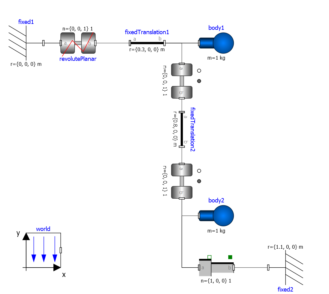
Figure 32 piston.mo

model piston
  Modelica.Mechanics.MultiBody.Parts.Fixed fixed1 annotation(
    Placement(visible = true, transformation(origin = {-80, 70}, extent = {{-10, -10}, {10, 10}}, rotation = 0)));
  Modelica.Mechanics.MultiBody.Parts.Body body1(m = 1)  annotation(
    Placement(visible = true, transformation(origin = {30, 70}, extent = {{-10, -10}, {10, 10}}, rotation = 0)));
  Modelica.Mechanics.MultiBody.Parts.FixedTranslation fixedTranslation1(r = {0.3, 0, 0})  annotation(
    Placement(visible = true, transformation(origin = {-10, 70}, extent = {{-10, -10}, {10, 10}}, rotation = 0)));
  Modelica.Mechanics.MultiBody.Parts.FixedTranslation fixedTranslation2(r = {0.8, 0, 0})  annotation(
    Placement(visible = true, transformation(origin = {10, 20}, extent = {{-10, -10}, {10, 10}}, rotation = -90)));
  Modelica.Mechanics.MultiBody.Parts.Fixed fixed2(animation = false, r = {1.1, 0, 0})  annotation(
    Placement(visible = true, transformation(origin = {70, -60}, extent = {{-10, -10}, {10, 10}}, rotation = 180)));
  Modelica.Mechanics.MultiBody.Parts.Body body2(m = 1)  annotation(
    Placement(visible = true, transformation(origin = {30, -30}, extent = {{-10, -10}, {10, 10}}, rotation = 0)));
  inner Modelica.Mechanics.MultiBody.World world annotation(
    Placement(visible = true, transformation(origin = {-70, -50}, extent = {{-10, -10}, {10, 10}}, rotation = 0)));
  Modelica.Mechanics.MultiBody.Joints.Prismatic prismatic(animation = true)  annotation(
    Placement(visible = true, transformation(origin = {30, -60}, extent = {{-10, -10}, {10, 10}}, rotation = 0)));
  Modelica.Mechanics.MultiBody.Joints.RevolutePlanarLoopConstraint revolutePlanar annotation(
    Placement(visible = true, transformation(origin = {-50, 70}, extent = {{-10, -10}, {10, 10}}, rotation = 0)));
  Modelica.Mechanics.MultiBody.Joints.Revolute revolute1(a(fixed = false),phi(fixed = false), w(fixed = false))  annotation(
    Placement(visible = true, transformation(origin = {10, 48}, extent = {{-10, -10}, {10, 10}}, rotation = -90)));
  Modelica.Mechanics.MultiBody.Joints.Revolute revolute2 annotation(
    Placement(visible = true, transformation(origin = {10, -10}, extent = {{-10, -10}, {10, 10}}, rotation = -90)));
equation
  connect(prismatic.frame_b, fixed2.frame_b) annotation(
    Line(points = {{40, -60}, {60, -60}, {60, -60}, {60, -60}}, color = {95, 95, 95}));
  connect(fixed1.frame_b, revolutePlanar.frame_a) annotation(
    Line(points = {{-70, 70}, {-60, 70}, {-60, 70}, {-60, 70}}));
  connect(revolutePlanar.frame_b, fixedTranslation1.frame_a) annotation(
    Line(points = {{-40, 70}, {-20, 70}, {-20, 70}, {-20, 70}}, color = {95, 95, 95}));
  connect(fixedTranslation1.frame_b, revolute1.frame_a) annotation(
    Line(points = {{0, 70}, {10, 70}, {10, 58}, {10, 58}}, color = {95, 95, 95}));
  connect(revolute1.frame_b, fixedTranslation2.frame_a) annotation(
    Line(points = {{10, 38}, {10, 38}, {10, 30}, {10, 30}}, color = {95, 95, 95}));
  connect(revolute2.frame_b, prismatic.frame_a) annotation(
    Line(points = {{10, -20}, {10, -20}, {10, -60}, {20, -60}, {20, -60}}));
  connect(revolute2.frame_b, body2.frame_a) annotation(
    Line(points = {{10, -20}, {10, -20}, {10, -30}, {20, -30}, {20, -30}}, color = {95, 95, 95}));
  connect(revolute2.frame_a, fixedTranslation2.frame_b) annotation(
    Line(points = {{10, 0}, {10, 0}, {10, 10}, {10, 10}}, color = {95, 95, 95}));
  connect(fixedTranslation1.frame_b, body1.frame_a) annotation(
    Line(points = {{0, 70}, {18, 70}, {18, 70}, {20, 70}}));
end piston;

>>> loadModel(Modelica);
>>> setCommandLineOptions("-d=initialization");
>>> buildModel(piston);
"[/var/lib/jenkins1/ws/OpenModelica_master_2/build/lib/omlibrary/Modelica 4.0.0+maint.om/Mechanics/MultiBody/Parts/Body.mo:14:3-15:65:writable] Warning: Parameter body1.r_CM has no value, and is fixed during initialization (fixed=true), using available start value (start={0, 0, 0}) as default value.
[/var/lib/jenkins1/ws/OpenModelica_master_2/build/lib/omlibrary/Modelica 4.0.0+maint.om/Mechanics/MultiBody/Parts/Body.mo:14:3-15:65:writable] Warning: Parameter body2.r_CM has no value, and is fixed during initialization (fixed=true), using available start value (start={0, 0, 0}) as default value.
Warning: Assuming fixed start value for the following 2 variables:
         $STATESET2.x:VARIABLE(start = /*Real*/($STATESET2.A[1]) * $START.revolute1.phi + /*Real*/($STATESET2.A[2]) * $START.revolute2.phi fixed = true )  type: Real
         $STATESET1.x:VARIABLE(start = /*Real*/($STATESET1.A[1]) * $START.revolute1.w + /*Real*/($STATESET1.A[2]) * $START.revolute2.w fixed = true )  type: Real
"

Note how OpenModelica will inform the user about relevant and irrelevant start values for this model and for which variables a fixed default start value is assumed. The model has four joints but only one degree of freedom, so one of the joints revolutePlanar or prismatic must be initialized.

So, initializing phi and w of revolutePlanar will give a sensible start system.

model pistonInitialize
  extends piston(revolute1.phi.fixed = true, revolute1.phi.start = -1.221730476396031, revolute1.w.fixed = true, revolute1.w.start = 5);
equation
end pistonInitialize;

>>> setCommandLineOptions("-d=initialization");
>>> simulate(pistonInitialize, stopTime=2.0);
"[/var/lib/jenkins1/ws/OpenModelica_master_2/build/lib/omlibrary/Modelica 4.0.0+maint.om/Mechanics/MultiBody/Parts/Body.mo:14:3-15:65:writable] Warning: Parameter body1.r_CM has no value, and is fixed during initialization (fixed=true), using available start value (start={0, 0, 0}) as default value.
[/var/lib/jenkins1/ws/OpenModelica_master_2/build/lib/omlibrary/Modelica 4.0.0+maint.om/Mechanics/MultiBody/Parts/Body.mo:14:3-15:65:writable] Warning: Parameter body2.r_CM has no value, and is fixed during initialization (fixed=true), using available start value (start={0, 0, 0}) as default value.
"

Figure 33 Vertical movement of mass body2.

Importing initial values from previous simulations

In many use cases it is useful to import initial values from previous simulations, possibly obtained with another Modelica tool, which are saved in a .mat file. There are two different options to do that.

Using previous simulation results as start values for the initial equations

The first option is to solve the initial equations specified by the Modelica model, using the previous simulation results as initial guesses for the iterative solvers, in case they are needed. This can be very helpful in case the initialization problem involves the solution of large nonlinear systems of equations by means of iterative algorithms, whose convergence is sensitive to the selected initial guess.

Importing a previously found solution allows the OpenModelica solver to pick very good initial guesses for the unknowns of the iterative solvers, thus achieving convergence with a few iterations. Since the initial equations are solved in the process, the values of all variables and derivatives, as well as of all parameters with fixed = false attribute, are re-computed and fully consistent with the selected initial conditions, even in case the previously saved simulation results refer to a slightly different model configuration. Note that parameters with fixed = true will also get their values from the imported .mat file, so if you want to change them you need to edit the .mat file accordingly.

This option is activated by selecting the simulation result file name in the OMEdit Simulation Setup | Simulation Flag | Equation System Initialization File input field, or by setting the additional simulation flag -iif=resultfile.mat. By activating the checkbox Save simulation flags inside the model i.e., __OpenModelica_simulationFlags annotation, a custom annotation __OpenModelica_simulationFlags(iif="filename.mat") is added to the model, so this setting is saved with the model and is reused when loading the model again later on. It is also possible to specify at which point in time of the saved simulation results the initial values should be picked, by means of the Simulation Setup | Simulation Flags | Equation System Initialization Time input field, or by setting the simulation flag -iit=initialTimeValue.

Using previous simulation results to directly initialize a simulation

The second option is to skip the solution of the initial equations entirely, directly starting the simulation with the imported start values. In this case, the initial equations of the model are ignored, and the initial values of all parameters and state variables are directly set to the values loaded from the .mat file. This option is useful to restart a simulation from the final state of a previous one, ignoring whatever initial conditions are declared in the Modelica model by either fixed = true attributes or initial equations.

Note that state variables and parameters will be directly initialized to the imported values, while algebraic variables will be recomputed with the regular simulation equations, on the basis of the imported initial state and parameter values. The values of algebraic variables in the imported file will only be used to initialize iteration variables, in case this computation involves nonlinear implicit equations and iterative solvers, otherwise they will be ignored.

To activate this second option, set Simulation Setup | Simulation Flag | Initialization Method to none in OMEdit, or set the simulation flag -iim=none. Also in this case, activating the checkbox Save simulation flags inside model, i.e. __OpenModelica_simulationFlags annotation saves this option in an __OpenModelica_simulationFlags(iim=none) annotation, so it is retained for future simulations of the same model.

Beware of missing variables in the simulation result file

When importing simulation results to initialize a new simulation, bear in mind that, by default, protected and hidden variables are not saved to the .mat file, so they will be missing when importing the simulation results for initialization. This is particularly dangerous when the imported values are used directly, as unsaved protected or hidden variables will not be initialized and will retain their default zero value, which is likely to cause numerical problems such as division by zero when the simulation is started.

To avoid this problem, make sure you also save protected and hidden variables in the simulation result file, by setting the corresponding checkboxes in the Simulation Setup | Output tab of OMEdit, or by setting the simulation flags -emit_protected and -ignoreHideResult.

Example of use

The following minimal working example demonstrates the use of the initial value import feature. You can create a new package ImportInitialValues in OMEdit, copy and paste its code from here, and then run the different models in it.

package ImportInitialValues "Test cases for importing initial values in OpenModelica"
  partial model Base "The mother of all models"
    Real v1, v2, x;
    parameter Real p1;
    parameter Real p2 = 2*p1;
    final Real p3 = 3*p1;
  end Base;

  model ResultFileGenerator "Dummy model for generating the initial.mat file"
    extends Base(p1 = 7, p2 = 10);
  equation
    v1 = 2.8;
    v2 = 10;
    der(x) = 0;
  initial equation
    x = 4;
  annotation(
    experiment(StopTime = 1),
    __OpenModelica_simulationFlags(r = "../initial.mat"));
  end ResultFileGenerator;

  model M "Relies on Modelica code only for initialization"
    extends Base(
      v1(start = 14),
      p1 = 1, p2 = 1);
  equation
    (v1 - 3)*(v1 + 10)*(v1 - 15) = 0;
    v2 = time;
    der(x) = -x;
  initial equation
    x = 6;
  end M;

  model M2 "Imports parameters and initial guesses only, solve initial equations"
    extends M;
  annotation(__OpenModelica_simulationFlags(iif = "../initial.mat"));
  end M2;

  model M3 "import parameters, initial guesses and initial states, skip initial equations"
    extends M;
  annotation(__OpenModelica_simulationFlags(iim = "none", iif = "../initial.mat"));
  end M3;
end ImportInitialValues;

Running the ResultFileGenerator model creates an initial.mat file with some initial values in the root OMEdit working directory: p1 = 7, p2 = 10, p3 = 21, v1 = 2.8, v2 = 10, x = 4, der(x) = 0. Note that the default directory when running simulations in OMEdit is a sub-directory named as the full model pathname, located in the working directory, so it is necessary to go up one directory to access the root working directory.

When running model M, the simulation process only relies on the initial and guess values provided by the Modelica source code. Regarding the parameter values, p1 = 1, p2 = 1, p3 = 3*p1 = 3; regarding v1, the implicit cubic equation is solved iteratively using the start value 14 as an initial guess, thus converging to the nearest solution v1 = 15. The other variable v2 can be computed explicitly, so there is no need of any guess value for it. Finally, the initial value of the state variable is set to x = 6 by the initial equations.

When running model M2, the values of the initial.mat file are imported to provide values for non-final parameters and guess values for the initial equations, which are solved starting from there. Hence, the imported parameter values p1 = 7 and p2 = 10 override the model's binding equations, that would set both to 1; on the other hand, the final parameter p3 is computed based on the final binding equation to p3 = p1*3 = 21. Regarding v1, the iterative solver converges to the solution closest to the imported start value of 2.8, i.e. v1 = 3, while v2 is computed explicitly, so it doesn't depend on the imported start value, which is ignored. The initial value of the state x = 6 is obtained by solving the initial equation, which is explicit and thus ignores the imported guess value x = 4.

Finally, when running model M3, parameters are handled like in the previous case, as well as the algebraic variables v1 and v2. However, in this case the solution of the initial equations is skipped, so the state variable gets its initial value x = 4 straight from the imported initial.mat file.

Homotopy Method

For complex start conditions OpenModelica can have trouble finding a solution for the initialization problem with the default Newton method.

Modelica offers the homotopy operator [3] to formulate actual and simplified expression for equations, with homotopy parameter going from 0 to 1:

OpenModelica has different solvers available for non-linear systems. Initializing with homotopy on the first try is default if a homotopy operator is used. It can be switched off with noHomotopyOnFirstTry. For a general overview see [SCO+11], [Sie12], for details on the implementation in OpenModelica see [OB13].

The homotopy methods distinguish between local and global methods meaning, if affects the entire initialization system or only local strong connected components. In addition the homotopy methods can use equidistant or and adaptive in [0,1].

Default order of methods tried to solve initialization system

If there is no homotopy in the model

• Solve without homotopy method.

If there is homotopy in the model or solving without homotopy failed

• Try global homotopy approach with equidistant .

The default homotopy method will do three global equidistant steps from 0 to 1 to solve the initialization system.

Several compiler and simulation flags influence initialization with homotopy: --homotopyApproach, -homAdaptBend, -homBacktraceStrategy, -homHEps, -homMaxLambdaSteps, -homMaxNewtonSteps, -homMaxTries, -homNegStartDir, -homotopyOnFirstTry, -homTauDecFac, -homTauDecFacPredictor, -homTauIncFac, -homTauIncThreshold, -homTauMax, -homTauMin, -homTauStart, -ils.

Algebraic Solvers

If the ODE system contains equations that need to be solved together, so called algebraic loops, OpenModelica can use a variety of different linear and non-linear methods to solve the equation system during simulation.

For the C runtime the linear solver can be set with -ls and the non-linear solver with -nls. There are dense and sparse solver available.

Linear solvers

• default : Lapack with totalpivot as fallback [ABB+99]

• lapack : Non-Sparse LU factorization using [ABB+99]

• lis : Iterative linear solver [Nis10]

• klu : Sparse LU factorization [Nat05]

• umfpack : Sparse unsymmetric multifrontal LU factorization [Dav04]

• totalpivot : Total pivoting LU factorization for underdetermined systems

Non-linear solvers

• hybrid : Modified Powell hybrid method from MINPACK [DJS96]

• kinsol : Combination of Newton-Krylov, Picard and fixed-point solver [T+98]

• newton : Newton-Raphson method [CK06]

• mixed : Homotopy with hybrid as fallback [Kel78] [BBOR15]

• homotopy : Damped Newton solver with fixed-point solver and Newton homotopy solver as fallbacks

In addition, there are further optional settings for the algebraic solvers available. A few of them are listed in the following:

General: -nlsLS

Newton: -newton -newtonFTol -newtonMaxStepFactor -newtonXTol

Sparse solver: -nlssMinSize -nlssMaxDensity

Enable logging: -lv=LOG_LS -lv=LOG_LS_V -lv=LOG_NLS -lv=LOG_NLS_V

References

[ABB+99] (1,2)

Edward Anderson, Zhaojun Bai, Christian Bischof, L Susan Blackford, James Demmel, Jack Dongarra, Jeremy Du Croz, Anne Greenbaum, Sven Hammarling, Alan McKenney, and others. LAPACK Users' guide. SIAM, 1999.

[BBOR15]

Bernhard Bachmann, W Braun, L Ochel, and V Ruge. Symbolical and numerical approaches for solving nonlinear systems. In Annual OpenModelica Workshop, volume 2015. 2015.

[CK06] (1,2)

Francois E. Cellier and Ernesto Kofman. Continuous System Simulation. Springer-Verlag New York, Inc., Secaucus, NJ, USA, 2006. ISBN 0387261028.

[DN10]

T. A. Davis and E. Palamadai Natarajan. Algorithm 907: klu, a direct sparse solver for circuit simulation problems. ACM Trans. Math. Softw., 37(3):36:1–36:17, September 2010. URL: http://doi.acm.org/10.1145/1824801.1824814, doi:10.1145/1824801.1824814.

[Dav04]

Timothy A Davis. Algorithm 832: umfpack v4. 3—an unsymmetric-pattern multifrontal method. ACM Transactions on Mathematical Software (TOMS), 30(2):196–199, 2004.

[DJS96]

John E Dennis Jr and Robert B Schnabel. Numerical methods for unconstrained optimization and nonlinear equations. SIAM, 1996.

[HNorsettW93]

E. Hairer, S. P. Nørsett, and G. Wanner. Solving Ordinary Differential Equations I: Nonstiff Problems. Springer-Verlag Berlin Heidelberg, 2nd rev. ed. 1993. corr. 3rd printing 2008 edition, 1993. ISBN 978-3-540-56670-0. doi:10.1007/978-3-540-78862-1.

[HNorsettW00]

E. Hairer, S.P. Nørsett, and G. Wanner. Solving Ordinary Differential Equations I Nonstiff problems. Springer, Berlin, second edition, 2000.

[HBG+05] (1,2)

A. C. Hindmarsh, P. N. Brown, K. E. Grant, S. L. Lee, R. Serban, D. E. Shumaker, and C. S. Woodward. SUNDIALS: suite of nonlinear and differential/algebraic equation solvers. ACM Transactions on Mathematical Software (TOMS), 31(3):363–396, 2005.

[Kel78]

Herbert B Keller. Global homotopies and newton methods. In Recent advances in numerical analysis, pages 73–94. Elsevier, 1978.

[KC19]

Christopher A. Kennedy and Mark H. Carpenter. Diagonally implicit runge–kutta methods for stiff odes. Applied Numerical Mathematics, 146:221–244, 2019. URL: https://www.sciencedirect.com/science/article/pii/S0168927419301801, doi:https://doi.org/10.1016/j.apnum.2019.07.008.

[Nat05]

Ekanathan Palamadai Natarajan. KLU–A high performance sparse linear solver for circuit simulation problems. PhD thesis, University of Florida, 2005.

[Nis10]

Akira Nishida. Experience in developing an open source scalable software infrastructure in japan. In International Conference on Computational Science and Its Applications, 448–462. Springer, 2010.

[OB13]

Lennart A Ochel and Bernhard Bachmann. Initialization of equation-based hybrid models within openmodelica. In Proceedings of the 5th International Workshop on Equation-Based Object-Oriented Modeling Languages and Tools; April 19; University of Nottingham; Nottingham; UK, number 084, 97–103. Linköping University Electronic Press, 2013.

[Pet82]

L.R. Petzold. Description of dassl: a differential/algebraic system solver. 1982.

[Sie12]

Michael Sielemann. Device-Oriented Modeling and Simulation in Aircraft Energy Systems Design. PhD thesis, TU Hamburg-Harburg, Germany, 2012. doi:10.15480/882.1111.

[SCO+11]

Michael Sielemann, Francesco Casella, Martin Otter, Christop Clauß, Jonas Eborn, Sven Erik Matsson, and Hans Olsson. Robust initialization of differential-algebraic equations using homotopy. In Proceedings of the 8th International Modelica Conference; March 20th-22nd; Technical Univeristy; Dresden; Germany, number 063, 75–85. Linköping University Electronic Press, 2011.

[T+98]

Allan G Taylor and others. User documentation for kinsol, a nonlinear solver for sequential and parallel computers. Technical Report, Lawrence Livermore National Lab., CA (United States), 1998.

Footnotes

[1]

DASPK Webpage

[2]

Cdaskr source

[3]

Modelica Association, Modelica® - A Unified Object-Oriented Language for Systems Modeling Language Specification - Version 3.4, 2017 - Section 3.7.2.4