Data Reconciliation
Objective of Data Reconciliation
The objective of data reconciliation is to use physical models to reduce the impact of measurement errors by decreasing measurement uncertainties and detecting faulty sensors. Data reconciliation is possible only when redundant measurements are available. Redundancy can be achieved by linking together the measured variables of interest using the physical laws that constrain them. This can be done with static Modelica models (models featuring algebraic equations only, no differential equations).
Defining the Data Reconciliation Problem in OpenModelica
Let us take the example of the Modelica model of a splitter.
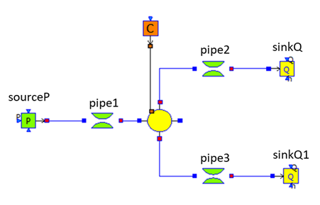
Water flows from left to right, from the source to the sinks. The model is made of five different model components.
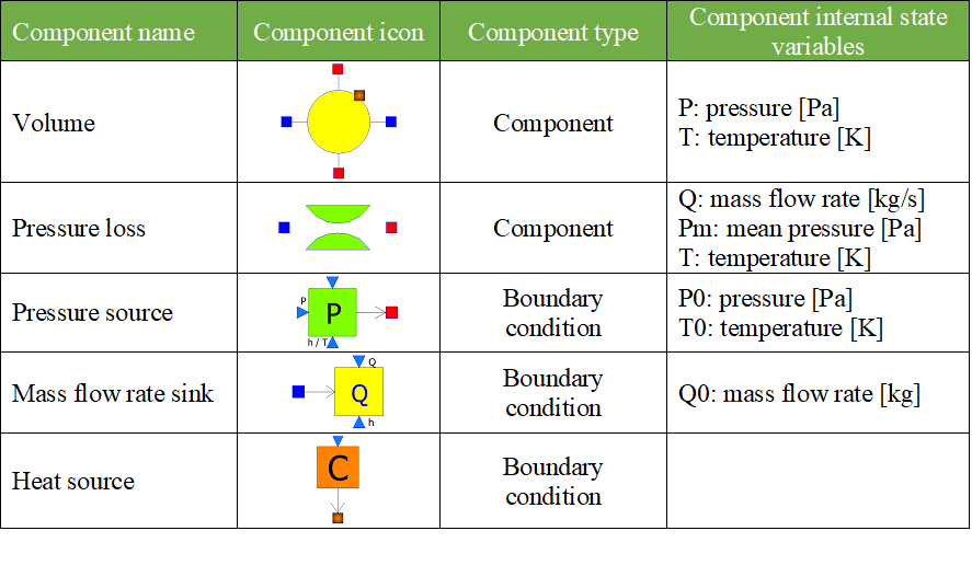
- To perform data reconciliation, two kinds of variables must be declared:
The boundary conditions (which represent assumptions on the environment);
The variables of interest to be reconciled.
- These two kinds of variables must be manually declared in the source code
With annotations for the boundary conditions;
With modifiers for the variables of interest.
The boundary conditions are declared with the annotation: annotation(__OpenModelica_BoundaryCondition = true). For the pressure source, the boundary conditions are the pressure P0, and the specific enthalpy h0 or the temperature T0 of the source (depending on the option chosen by the user).
model SourceP "Water/steam source with fixed pressure"
  parameter Modelica.SIunits.AbsolutePressure P0=300000 "Source pressure" annotation(__OpenModelica_BoundaryCondition = true);
  parameter Modelica.SIunits.Temperature T0=290 "Source temperature (active if option_temperature=1" annotation(__OpenModelica_BoundaryCondition = true);
  parameter Modelica.SIunits.SpecificEnthalpy h0=100000
    "Source specific enthalpy (active if option_temperature=2)" annotation(__OpenModelica_BoundaryCondition = true);
  parameter Integer option_temperature=1 "1:temperature fixed - 2:specific enthalpy fixed";

  Modelica.SIunits.AbsolutePressure P "Fluid pressure";
  Modelica.SIunits.MassFlowRate Q "Mass flow rate";
  Modelica.SIunits.Temperature T "Fluid temperature";
  Modelica.SIunits.SpecificEnthalpy h "Fluid enthalpy";
equation
  P = P0;
  if (option_temperature == 1) then
    T = T0;
     h = f(T);
  else
    h = h0;
    T = g(h);
  end if;
end SourceP;
Boundary conditions are declared with annotations so that libraries can be modified to accomodate data reconciliation, and still can be used with tools that do not support data reconciliation (because annotations not recognized by a tool are ignored by that tool). The variables of interest are declared with the modifier "uncertain = Uncertainty.refine"
A modifier is used instead of an annotation so that checks can be performed to detect errors such as declaring a variable that does not exist to be a variable to be reconciled. The drawback is that tools that do not support data reconciliation will produce an error. To avoid this problem, variables of interest should be declared in a separate model (Splitter_DR in the example below) that instantiates the orginal model (Splitter), so that the original model (Splitter) is not modified and can still be used with tools that do not support data reconciliation.
model Splitter_DR
  Splitter splitter(
     pipe1(Q(uncertain = Uncertainty.refine)),
     pipe2(Q(uncertain = Uncertainty.refine)),
     pipe3(Q(uncertain = Uncertainty.refine)),
     pipe1(Pm(uncertain = Uncertainty.refine)),
     pipe2(Pm(uncertain = Uncertainty.refine)),
     pipe3(Pm(uncertain = Uncertainty.refine)),
     pipe1(T(uncertain = Uncertainty.refine)),
     pipe2(T(uncertain = Uncertainty.refine)),
     pipe3(T(uncertain = Uncertainty.refine)));
end Splitter_DR;
- In addition to declaring boundary conditions and variables of interest, one must provide two input files:
The measurement input file (mandatory).
The correlation matrix input file (optional).
- The measurement input file is a csv file with three columns:
One column for the variable names [ident]
One column for measured values [positive floating point number]
One column for the half-width confidence intervals [positive floating point number].The half-with confidence interval for variable
 is defined as
  , where
  is the standard deviation of and
- The header of the file is the row
- Variable Names; Measured Value-x; Half Width Confidence Interval
- It is possible to insert comments with // at the beginning of a row
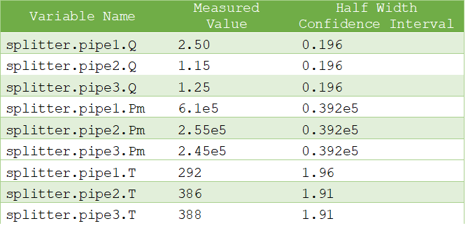
- // Measurement input file for the Splitter model.Variable Name;Measured Value;Half Width Confidence Intervalsplitter.pipe1.Q; 2.50; 0.196splitter.pipe2.Q; 1.15; 0.196splitter.pipe3.Q; 1.25; 0.196splitter.pipe1.Pm; 6.1e5; 0.392e5splitter.pipe2.Pm; 2.55e5; 0.392e5splitter.pipe3.Pm; 2.45e5; 0.392e5splitter.pipe1.T; 292; 1.96splitter.pipe2.T; 386; 1.91splitter.pipe3.T; 388; 1.91
The above file can be more easily visualized in matrix form:
The correlation matrix file is a csv file that contains the off-diagonal lower triangular correlation coefficients of the variables of interest:
The first row contains names of variables of interest [ident].
The first column contains names of variables of interest [ident].
The names in the first row and first column must be identical in the same order.
The first cell in the first row (which is also the first cell in the first column) must not be empty, but can contain any character string (except column separators).
The off-diagonal lower triangular matrix cells contain the correlation coefficients [positive or nul floating point number]. The correlation coefficients
are defined such that
where
are respectively the standard deviations of variables
, and
is the covariance matrix.
because
The upper triangular and diagonal cells are ignored because the correlation matrix is symmetric
, and its diagonal is
Only variables of interest with positive correlation coefficients must appear in the matrix. Unfilled cells are equal to zero. Variables of interest that do not appear in the matrix have correlation coefficients equal to zero. Therefore, if all correlation coefficients are equal to zero, the matrix can be empty and the correlation matrix file is not needed

The following correlation file is drawn from the VDI2048 standard example of a heat circuit of a steam turbine plant.
Sxy;mV;mHK;mSPLL;mSPL;mFDKELL;mFDKELmVmHKmSPLLmSPL;;;0.39951mFDKELL;;;0;0mFDKEL;;;0;0;0.2
The above file can be more easily visualized in matrix form:
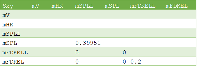
The variables mV and mHK could have been omitted because they do not have any positive correlation coefficients.
Data Reconciliation Support in OMEdit
- The data reconciliation setup is done by:
Opening the Modelica model with the data reconciliation modifiers in OMEdit.
Selecting Data Reconciliation > Calculate Data Reconciliation.
Selecting the Data Reconciliation algorithm.
- Filling the Data Reconciliation form with
The name of the Measurement Input File (mandatory);
The name of the Correlation Matrix Input file (optional). The default is the identity matrix (i.e. measurements are independent of each other);
The value of Epsilon (optional). The default value is 1.e-10. Epsilon is the stopping criteria of the data reconciliation numerical iterations.
Clicking on Save Settings to save the above settings in the Modelica model.
Clicking on Calculate to launch the calculation
- The data reconciliation computation is performed in three main steps:
- Static analysis is performed on the model to extract the equations that are necessary for data reconciliation. There are two groups of extracted equations:
The auxiliary conditions that constrain the variables of interest.
The intermediate equations that solve the intermediate variables from the variables of interest (this is the numeric way of eliminating the intermediate variables).
The auxiliary and intermediate equations are interchangeable: denoting r the number of auxiliary conditions, there are as many possibilities to construct the set of auxiliary conditions as to choose r equations among the set that contains both the auxiliary and the intermediate equations.
- Any error in the posing of the data reconciliation problem is detected at this step. The possible errors are:
The number r of auxiliary equations is not strictly less than the number of variables of interest.
The number r of auxiliary equations is zero.
Both errors occur when there are too many boundary conditions related to the variables of interest. Variables of interest that are not involved in any of the auxiliary conditions or intermediate equations are not reconciled.
The model is simulated to compute the Jacobian matrices and eliminate numerically the intermediate variables. At this step, numerical simulation errors can occur, such as divisions by zero, non-convergence, etc. They can be corrected by improving the model or providing better start values.
- The input files are read, the data reconciliation calculation is performed, and the results are displayed. Errors can occur:
If input files do not exist.
- If there is a mismatch between the variables of interest declared in the model and in the input files:
All variables of interest declared in the model should be declared in the measurement input file and reciprocally.
All variables of interest declared in the correlation matrix file should be declared in the model (the converse is not true).
If a variable of interest has multiple entries in an input file.
If the first row and the first column are different in the correlation matrix file.
If the numerical cells of the matrices are not positive real numbers.
- The results are displayed:
In an html file with the title: Data Reconciliation Report. This file automatically pops up when the calculation is completed.
- In two csv output files:
One that contains the reconciled values and the reconciled half-width confidence intervals.
The other that contains the reconciled covariance matrix.
- These files do not pop up automatically when the calculation is completed. The names of the files are respectively
- <working directory>\<model name>\< model name>_Outputs.csv
- and
- <working directory>\<model name>\< model name>_Reconciled_Sx.csv,
where <model name> denotes the full name of the model, including its path. The name of the working directory can be read with the command Tools > Options.
The Data Reconciliation Report has three sections:
- Overview, with the following information:
Model file: name of the Modelica model file
Model name: name of the Modelica model
Model directory: name of the directory of the Modelica model file
Measurement input file: name of the measurement input file
Correlation matrix input file: name of the correlation matrix file (if any)
Generated: date and time of the generation of the data reconciliation report
- Analysis, with the following information:
Number of auxiliary conditions, denoted r in the sequel.
Number of variables to be reconciled.
Number of related boundary conditions: number of boundary conditions related to the variables to be reconciled. This number should be strictly less than the number of variables to be reconciled, otherwise the data reconciliation problem is ill-posed and data reconciliation cannot be performed.
Number of iterations to convergence: number of iterations of the data reconciliation numerical loop.
Final value of J*/r: final value of the data reconciliation iteration loop. This value is smaller than epsilon when the iterations are completed (cf. below).
Epsilon: stopping criteria of the data reconciliation iteration loop. The recommended value by VDI 2048 is 1.e-10.
Final value of the objective function J*: is equal to J*/r multiplied by r, where r is the number of auxiliary conditions.
Chi-square value: value of the chi-square distribution for r degrees of freedom and statistical certainty of probability of 95%.
Result of global test: true if J* is less than the chi-square value, false otherwise. If false, the results for the reconciled values should be rejected because the vector of contradictions (i.e. the discrepancy between the measured values and the reconciled values) is too large.
Auxiliary conditions: set of the auxiliary conditions (i.e., the equations that constrain the variables of interest).
Intermediate equations: set of the intermediate equations (i.e., the equations that compute the intermediate variables from the variables of interest). This set can be empty if there are no intermediate variables.
Debug log: log of the numerical iteration loop.
- Results, which is a table with the following columns:
Variables to be Reconciled: the names of the variables of interest.
Initial Measured Values: the measured values entered in the measurement input file.
Reconciled Values: the reconciled values computed by the data reconciliation algorithm.
Initial Half-width Confidence Intervals: the half-width confidence intervals entered in the measurement input file.
Reconciled Half-width Confidence Intervals: the reconciled half-width confidence intervals computed by the data reconciliation algorithm.
Results of Local Tests: true if the values of local tests (cf. below) are less than the quantile of normal distribution with probability 95% (
), false otherwise.
Values of Local Tests: values of the improvements (i.e., the difference between the initial and the reconciled values) divided by the square root of the diagonal element of the covariance matrix of the improvements.
Margin to Correctness:
The data reconciliation report for the the VDI2048 standard example of a heat circuit of a steam turbine plant is given below.
Overview:
Model file: VDI2048Example.moModel name: NewDataReconciliationSimpleTests.VDI2048ExampleModel directory: NewDataReconciliationSimpleTestsMeasurement input file: VDI2048Example_Inputs.csvCorrelation matrix input file: VDI2048Example_Correlation.csvGenerated: Thu Jan 20 18:41:45 2022by OpenModelica v1.19.0-dev-500-g6c3a4e429f (64-bit)
Analysis:
Number of auxiliary conditions: 3Number of variables to be reconciled: 11Number of related boundary conditions: 0Number of iterations to convergence: 2Final value of (J*/r) : 4.56744e-28Epsilon : 1e-10Final value of the objective function (J*) : 1.37023e-27Chi-square value : 7.81473Result of global test : TRUE
Auxiliary conditions
(1): 0.0 = mHDANZ - mHDNK
(1): mFD3 = mHK + mA7 + mA6 + mA5 + 0.4 * mV
(1): mFD1 = mFDKEL + mFDKELL + (-0.2) * mV
Intermediate equations
(1): mHDANZ = mA7 + mA6 + mA5
(1): mFD2 = mSPL + mSPLL + (-0.6) * mV
(1): 0.0 = mFD2 - mFD3
(1): 0.0 = mFD1 - mFD2
Debug log
Results
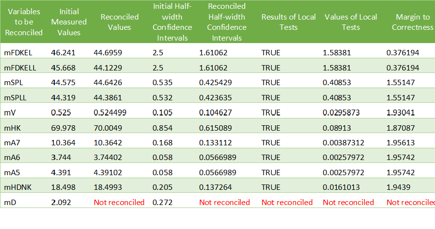
mD is not reconciled because it does not appear in any of the auxiliary conditions or intermediate equations.
- For the VDI2048 example, the name of the csv output file is
- <working directory>\NewDataReconciliationSimpleTests.VDI2048Example\NewDataReconciliationSimpleTests.VDI2048Example_Outputs.csv
- and the name of the reconciled covariance matrix csv file is
- <working directory>\NewDataReconciliationSimpleTests.VDI2048Example\NewDataReconciliationSimpleTests.VDI2048Example_ Reconciled_Sx.csv
The Modelica model of the VDI2048 example is given below.
model VDI2048Example
  Real mFDKEL(uncertain=Uncertainty.refine)=46.241;
  Real mFDKELL(uncertain=Uncertainty.refine)=45.668;
  Real mSPL(uncertain=Uncertainty.refine)=44.575;
  Real mSPLL(uncertain=Uncertainty.refine)=44.319;
  Real mV(uncertain=Uncertainty.refine);
  Real mHK(uncertain=Uncertainty.refine)=69.978;
  Real mA7(uncertain=Uncertainty.refine)=10.364;
  Real mA6(uncertain=Uncertainty.refine)=3.744;
  Real mA5(uncertain=Uncertainty.refine);
  Real mHDNK(uncertain=Uncertainty.refine);
  Real mD(uncertain=Uncertainty.refine)=2.092;
  Real mFD1;
  Real mFD2;
  Real mFD3;
  Real mHDANZ;
equation
  mFD1 = mFDKEL + mFDKELL - 0.2*mV;
  mFD2 = mSPL + mSPLL - 0.6*mV;
  mFD3 = mHK + mA7 + mA6 + mA5 + 0.4*mV;
  mHDANZ = mA7 + mA6 + mA5;

  0 = mFD1 - mFD2;
  0 = mFD2 - mFD3;
  0 = mHDANZ - mHDNK;
end VDI2048Example;
Note that the binding equations that assign fixed values to the variables have been automatically eliminated by the extraction algorithm. These equations are necessary to have a valid square Modelica model, but must be eliminated for data reconciliation.
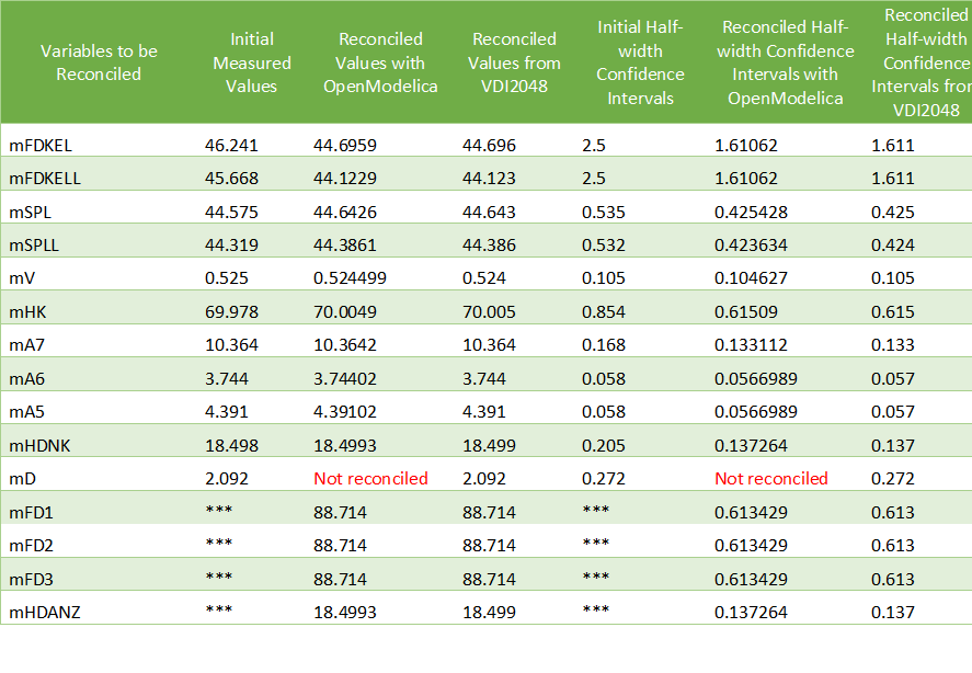
The table below compares the results obtained with OpenModelica with those given by the VDI2048 standard.
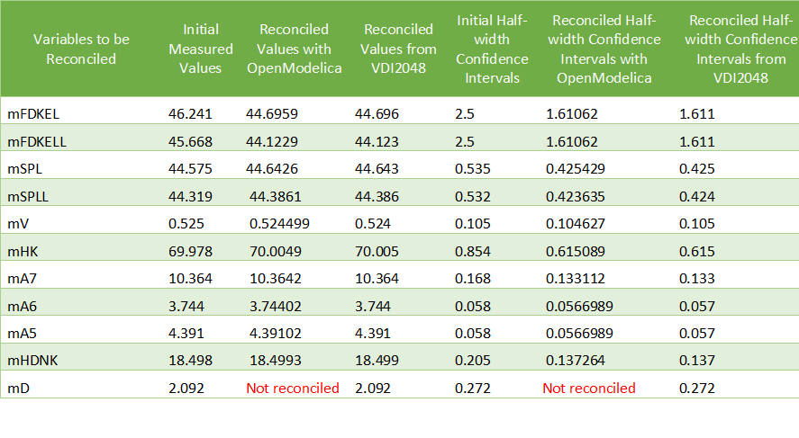
The value of mD is left unchanged after reconciliation. This is indicated by 'Not reconciled' in OpenModelica, and by repeating the initial measured values in VDI2048. In order to compute the reconciled values of mFD1, mFD2, mFD3 and mHDANZ, which have no measurements, it is possible to consider them as variables of interest with very large half-width confidence, e.g., 1e4, and assign them arbitrary measured values, e.g. 0. The result is
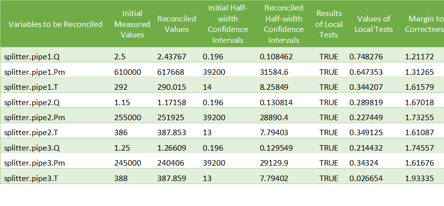
For the splitter, the results are the following:
Computing the Boundary Conditions from the Reconciled Values
- The values and uncertainties of the boundary conditions that correspond to the reconciled values of the variables of interest can be computed by:
Selecting Data Reconciliation > Calculate Data Reconciliation
Selecting the Boundary Conditions algorithm.
- Filling the Data Reconciliation form with
The name of the Reconciled Measurement File (mandatory). It is the name of the csv output file produced by the data reconciliation algorithm.
The name of the Reconciled Correlation Matrix file (mandatory). It is the name of the correlation matrix csv file produced by the data reconciliation algorithm.
Clicking on Save Settings to save the above settings in the Modelica model.
Clicking on Calculate to launch the calculation.
- At least one boundary condition must be declared in the model, otherwise the computation fails with a difficult to interpret error message such as
- Cannot Compute Jacobian Matrix F.
A better error message will be posted in a future version.
- The computation of the boundary conditions is performed in three main steps:
- Static analysis is performed on the model to extract the equations that compute the boundary conditions from the variables of interest. This corresponds to automatically inverting the original model. There are two groups of extracted equations:
The boundary conditions that are the equations that compute the boundary conditions.
The intermediate equations that solve the intermediate variables from the variables of interest (this is the numeric way of eliminating the intermediate variables).
2. The model is simulated to compute the Jacobian matrices and eliminate numerically the intermediate equations. At this step, numerical simulation errors can occur, such as divisions by zero, non-convergence, etc. They can be corrected by improving the model or providing better start values.
The input files are read, the numerical calculations are performed, and the results are displayed. The half-width confidence intervals for the boundary conditions are calculated by propagating the reconciled uncertainties on the variables of interest through the inverted model.
- The results are displayed:
In an html file with the title: Boundary Condition Report. This file pops up automatically when the calculation is completed.
2. In a csv output file. The name of the csv output file is <working directory>\<model name>\< model name>_ BoundaryConditions_Outputs.csv
The Boundary Condition Report has three sections:
Overview
Model file: name of the Modelica model file
Model name: name of the Modelica model
Model directory: name of the directory of the Modelica model file
Reconciled values input file: name of the csv output file produced by the data reconciliation algorithm
Reconciled covariance matrix input file: name of the correlation matrix csv file produced by the data reconciliation algorithm
Generated: date and time of the generation of the boundary condition report
Analysis
Number of boundary conditions.
Number of reconciled variables.
Boundary conditions: set of the boundary conditions (i.e., the equations that compute the boundary conditions).
Intermediate equations: set of the intermediate equations (i.e., the equations that compute the intermediate variables from the variables of interest).
Debug log
Log of the numerical iteration loop
Results
- A table with the following columns
Boundary Conditions: the names of the boundary conditions.
Values: the computed values of the boundary conditions.
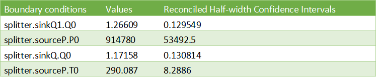
Reconciled Half-width Confidence Intervals: the half-with confidence intervals for the boundary conditions.
The results for the splitter are:
Contacts
References
Bouskela, D., Jardin, A., Palanisamy, A., Ochel, L., & Pop, A. (2021). New Method to Perform Data Reconciliation with OpenModelica and ThermoSysPro. Proceedings of 14th Modelica Conference 2021, Linköping, Sweden, September 20-24, 2021.
VDI - Verein Deutscher Ingenieure. (2000). Uncertainty of measurement during acceptance tests on energy-conversion and power plants - Part 1: Fundamentals. VDI 2048 Blatt 1, October 2000.
