Optimization with OpenModelica

The following facilities for model-based optimization are provided with OpenModelica:

• Builtin Dynamic Optimization with OpenModelica and IpOpt using

  dynamic optimization is the recommended way of performing dynamic optimization with OpenModelica.

• Dynamic Optimization with OpenModelica and CasADi. Use this if you want to employ

  the CasADi tool for dynamic optimization.

• Classical Parameter Sweep Optimization using OMOptim. Use

  this if you have a static optimization problem.

Builtin Dynamic Optimization with OpenModelica and IpOpt

Note: this is a very short preliminary decription which soon will be considerably improved.

OpenModelica provides builtin dynamic optimization of models by using the powerful symbolic machinery of the OpenModelica compiler for more efficient and automatic solution of dynamic optimization problems.

The builtin dynamic optimization allows users to define optimal control problems (OCP) using the Modelica language for the model and the optimization language extension called Optimica (currently partially supported) for the optimization part of the problem. This is used to solve the underlying dynamic optimization model formulation using collocation methods, using a single execution instead of multiple simulations as in the parameter-sweep optimization described in section Parameter Sweep Optimization using OMOptim.

For more detailed information regarding background and methods, see [BOR+12][RBB+14]

Compiling the Modelica code

Before starting the optimization the model should be symbolically instantiated by the compiler in order to get a single flat system of equations. The model variables should also be scalarized. The compiler frontend performs this, including syntax checking, semantics and type checking, simplification and constant evaluation etc. are applied. Then the complete flattened model can be used for initialization, simulation and last but not least for model-based dynamic optimization.

The OpenModelica command optimize(ModelName) from OMShell, OMNotebook or MDT runs immediately the optimization. The generated result file can be read in and visualized with OMEdit or within OMNotebook.

An Example

In this section, a simple optimal control problem will be solved. When formulating the optimization problems, models are expressed in the Modelica language and optimization specifications. The optimization language specification allows users to formulate dynamic optimization problems to be solved by a numerical algorithm. It includes several constructs including a new specialized class optimization, a constraint section, startTime, finalTime etc. See the optimal control problem for batch reactor model below.

Create a new file named BatchReactor.mo and save it in you working directory. Notice that this model contains both the dynamic system to be optimized and the optimization specification.

Once we have formulated the undelying optimal control problems, we can run the optimization by using OMShell, OMNotebook, MDT, OMEdit using command line terminals similar to the options described below:

>>> setCommandLineOptions("-g=Optimica");

Listing 3 BatchReactor.mo

optimization BatchReactor(objective=-x2(finalTime), startTime = 0, finalTime =1)
  Real x1(start =1, fixed=true, min=0, max=1);
  Real x2(start =0, fixed=true, min=0, max=1);
  input Real u(min=0, max=5);
equation
  der(x1) = -(u+u^2/2)*x1;
  der(x2) = u*x1;
end BatchReactor;

optimization nmpcBatchReactor(objective=-x2)
  extends BatchReactor;
end nmpcBatchReactor;

>>> optimize(nmpcBatchReactor, numberOfIntervals=16, stopTime=1, tolerance=1e-8)
record SimulationResult
    resultFile = "«DOCHOME»/nmpcBatchReactor_res.mat",
    simulationOptions = "startTime = 0.0, stopTime = 1.0, numberOfIntervals = 16, tolerance = 1e-08, method = 'optimization', fileNamePrefix = 'nmpcBatchReactor', options = '', outputFormat = 'mat', variableFilter = '.*', cflags = '', simflags = ''",
    messages = "stdout            | info    | The initialization finished successfully without homotopy method.

Optimizer Variables
========================================================
State[0]:x1(start = 1, nominal = 1, min = 0, max = 1, init = 1)
State[1]:x2(start = 0, nominal = 1, min = 0, max = 1, init = 0)
Input[2]:u(start = 0, nominal = 5, min = 0, max = 5)
--------------------------------------------------------
number of nonlinear constraints: 0
========================================================

******************************************************************************
This program contains Ipopt, a library for large-scale nonlinear optimization.
 Ipopt is released as open source code under the Eclipse Public License (EPL).
         For more information visit http://projects.coin-or.org/Ipopt
******************************************************************************

stdout            | info    | The simulation finished successfully.
",
    timeFrontend = 0.07025218800000001,
    timeBackend = 0.008228969000000001,
    timeSimCode = 0.03977739299999994,
    timeTemplates = 0.0235654,
    timeCompile = 0.327357918,
    timeSimulation = 0.030821688,
    timeTotal = 0.500093836
end SimulationResult;

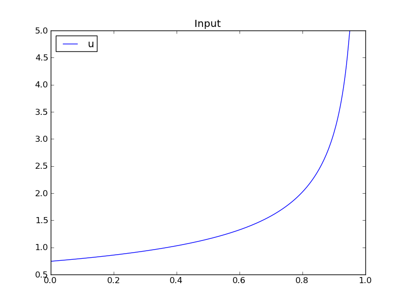
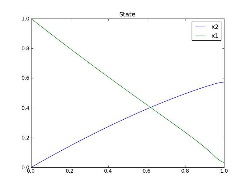
The control and state trajectories of the optimization results:

Figure 61 Optimization results for Batch Reactor model – input variables.

Figure 62 Optimization results for Batch Reactor model – state variables.

Different Options for the Optimizer IPOPT

Table 1 New meanings of the usual simualtion options for Ipopt.

numberOfIntervals		collocation intervals
startTime, stopTime		time horizon
tolerance = 1e-8	e.g. 1e-8	solver tolerance
simflags	all run/debug options

Table 2 New simulation options for Ipopt.

-lv	LOG_IPOPT	console output
-ipopt_hesse	CONST,BFGS,NUM	hessian approximation
-ipopt_max_iter	number e.g. 10	maximal number of iteration for ipopt
externalInput.csv		input guess

Dynamic Optimization with OpenModelica and CasADi

OpenModelica coupling with CasADi supports dynamic optimization of models by OpenModelica exporting the optimization problem to CasADi which performs the optimization. In order to convey the dynamic system model information between Modelica and CasADi, we use an XML-based model exchange format for differential-algebraic equations (DAE). OpenModelica supports export of models written in Modelica and the Optimization language extension using this XML format, while CasADi supports import of models represented in this format. This allows users to define optimal control problems (OCP) using Modelica and Optimization language specifications, and solve the underlying model formulation using a range of optimization methods, including direct collocation and direct multiple shooting.

Compiling the Modelica code

Before exporting a model to XML, the model should be symbolically instantiated by the compiler in order to get a single flat system of equations. The model variables should also be scalarized. The compiler frontend performs this, including syntax checking, semantics and type checking, simplification and constant evaluation etc. are applied. Then the complete flattened model is exported to XML code. The exported XML document can then be imported to CasADi for model-based dynamic optimization.

The OpenModelica command translateModelXML(ModelName) from OMShell, OMNotebook or MDT exports the XML. The export XML command is also integrated with OMEdit. Select XML > Export XML the XML document is generated in the current directory of omc. You can use the cd() command to see the current location. After the command execution is complete you will see that a file ModelName.xml has been exported.

Assuming that the model is defined in the modelName.mo, the model can also be exported to an XML code using the following steps from the terminal window:

• Go to the path where your model file found
• Run command omc -g=Optimica --simCodeTarget=XML Model.mo

An example

In this section, a simple optimal control problem will be solved. When formulating the optimization problems, models are expressed in the Modelica language and optimization specifications. The optimization language specification allows users to formulate dynamic optimization problems to be solved by a numerical algorithm. It includes several constructs including a new specialized class optimization, a constraint section, startTime, finalTime etc. See the optimal control problem for batch reactor model below.

Create a new file named BatchReactor.mo and save it in you working directory. Notice that this model contains both the dynamic system to be optimized and the optimization specification.

>>> list(BatchReactor)
optimization BatchReactor
  Real x1(start = 1, fixed = true, min = 0, max = 1);
  Real x2(start = 0, fixed = true, min = 0, max = 1);
  input Real u(min = 0, max = 5);
equation
  der(x1) = -(u + u ^ 2 / 2) * x1;
  der(x2) = u * x1;
end BatchReactor;

One we have formulated the undelying optimal control problems, we can export the XML by using OMShell, OMNotebook, MDT, OMEdit or command line terminals which are described in Section XML Import to CasADi via OpenModelica Python Script.

To export XML, we set the simulation target to XML:

>>> translateModelXML(BatchReactor)

Error

Error: Internal error - BackendDAE.incidenceRow failed for equation: $OMC$objectMayerTerm := -x2(finalTime)

Error: Internal error BackendDAEUtil.incidenceMatrix failed.

Error: pre-optimization module removeEqualFunctionCalls (simulation) failed.

Error: Internal error SimCode: The model BatchReactor could not be translated to XML

Error: Internal error - BackendDAE.incidenceRow failed for equation: $OMC$objectMayerTerm := -x2(finalTime)

Error: Internal error BackendDAEUtil.incidenceMatrix failed.

Error: pre-optimization module removeEqualFunctionCalls (simulation) failed.

Error: Internal error SimCode: The model BatchReactor could not be translated to XML

This will generate an XML file named batchreactorxml (batchreactorxml) that contains a symbolic representation of the optimal control problem and can be inspected in a standard XML editor.

XML Import to CasADi via OpenModelica Python Script

The symbolic optimal control problem representation (or just model description) contained in BatchReactor.xml can be imported into CasADi in the form of the SymbolicOCP class via OpenModelica python script.

The SymbolicOCP class contains symbolic representation of the optimal control problem designed to be general and allow manipulation. For a more detailed description of this class and its functionalities, we refer to the API documentation of CasADi.

The following step compiles the model to an XML format, imports to CasADi and solves an optimization problem in windows PowerShell:

1. Create a new file named BatchReactor.mo and save it in you working directory.

   E.g. C:\OpenModelica1.9.2\share\casadi\testmodel

1. Perform compilation and generate the XML file

   1. Go to your working directory

   E.g. cd C:\OpenModelica1.9.2\share\casadi\testmodel

1. Go to omc path from working directory and run the following command

   E.g. ..\..\..\bin\omc +s -g=Optimica --simCodeTarget=XML BatchReactor.mo

3. Run defaultStart.py python script from OpenModelica optimization directory

E.g. Python.exe ..\share\casadi\scripts defaultStart.py BatchReactor.xml

The control and state trajectories of the optimization results are shown below:

Parameter Sweep Optimization using OMOptim

OMOptim is a tool for parameter sweep design optimization of Modelica models. By optimization, one should understand a procedure which minimizes/maximizes one or more objective functions by adjusting one or more parameters. This is done by the optimization algorithm performing a parameter swep, i.e., systematically adjusting values of selected parameters and running a number of simulations for different parameter combinations to find a parameter setting that gives an optimal value of the goal function.

OMOptim 0.9 contains meta-heuristic optimization algorithms which allow optimizing all sorts of models with following functionalities:

• One or several objectives optimized simultaneously
• One or several parameters (integer or real variables)

However, the user must be aware of the large number of simulations an optimization might require.

Preparing the Model

Before launching OMOptim, one must prepare the model in order to optimize it.

Parameters

An optimization parameter is picked up from all model variables. The choice of parameters can be done using the OMOptim interface.

For all intended parameters, please note that:

• The corresponding variable is constant during all simulations.

  The OMOptim optimization in version 0.9 only concerns static parameters’ optimization i.e. values found for these parameters will be constant during all simulation time.

• The corresponding variable should play an input role in the model

  i.e. its modification influences model simulation results.

Constraints

If some constraints should be respected during optimization, they must be defined in the Modelica model itself.

For instance, if mechanical stress must be less than 5 N.m^-2, one should write in the model:

assert(mechanicalStress < 5, "Mechanical stress too high");

If during simulation, the variable mechanicalStress exceeds 5 N.m^-2, the simulation will stop and be considered as a failure.

Objectives

As parameters, objectives are picked up from model variables. Objectives’ values are considered by the optimizer at the final time.

Set problem in OMOptim

Launch OMOptim

OMOptim can be launched using the executable placed in OpenModelicaInstallationDirectory/bin/ OMOptim/OMOptim.exe. Alternately, choose OpenModelica > OMOptim from the start menu.

Create a new project

To create a new project, click on menu File -> New project

Then set a name to the project and save it in a dedicated folder. The created file created has a .min extension. It will contain information regarding model, problems, and results loaded.

Load models

First, you need to load the model(s) you want to optimize. To do so, click on Add .mo button on main window or select menu Model -> Load Mo file…

When selecting a model, the file will be loaded in OpenModelica which runs in the background.

While OpenModelica is loading the model, you could have a frozen interface. This is due to multi-threading limitation but the delay should be short (few seconds).

You can load as many models as you want.

If an error occurs (indicated in log window), this might be because:

• Dependencies have not been loaded before (e.g. modelica library)
• Model use syntax incompatible with OpenModelica.

Dependencies

OMOptim should detect dependencies and load corresponding files. However, it some errors occur, please load by yourself dependencies. You can also load Modelica library using Model->Load Modelica library.

When the model correctly loaded, you should see a window similar to Figure 63.

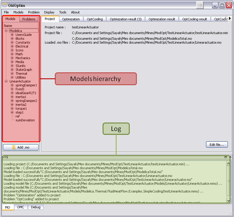
Figure 63 OMOptim window after having loaded model.

Create a new optimization problem

Problem->Add Problem->Optimization

A dialog should appear. Select the model you want to optimize. Only Model can be selected (no Package, Component, Block…).

A new form will be displayed. This form has two tabs. One is called Variables, the other is called Optimization.

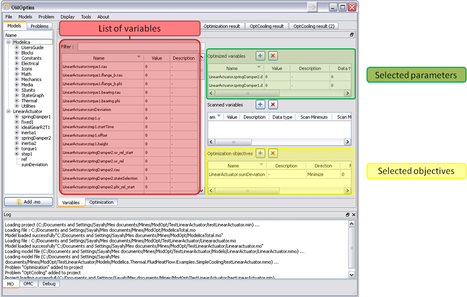
Figure 64 Forms for defining a new optimization problem.

List of Variables is Empty

If variables are not displayed, right click on model name in model hierarchy, and select Read variables.

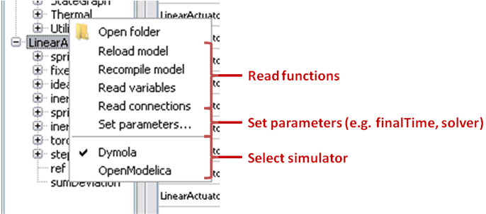
Figure 65 Selecting read variables, set parameters, and selecting simulator.

Select Optimized Variables

To set optimization, we first have to define the variables the optimizer will consider as free i.e. those that it should find best values of. To do this, select in the left list, the variables concerned. Then, add them to Optimized variables by clicking on corresponding button ().

For each variable, you must set minimum and maximum values it can take. This can be done in the Optimized variables table.

Select objectives

Objectives correspond to the final values of chosen variables. To select these last, select in left list variables concerned and click button of Optimization objectives table.

For each objective, you must:

• Set minimum and maximum values it can take. If a configuration does

  not respect these values, this configuration won’t be considered. You also can set minimum and maximum equals to “-“ : it will then

• Define whether objective should be minimized or maximized.

This can be done in the Optimized variables table.

Select and configure algorithm

After having selected variables and objectives, you should now select and configure optimization algorithm. To do this, click on Optimization tab.

Here, you can select optimization algorithm you want to use. In version 0.9, OMOptim offers three different genetic algorithms. Let’s for example choose SPEA2Adapt which is an auto-adaptative genetic algorithm.

By clicking on parameters… button, a dialog is opened allowing defining parameters. These are:

• Population size: this is the number of configurations kept after a

  generation. If it is set to 50, your final result can’t contain more than 50 different points.

• Off spring rate: this is the number of children per adult obtained

  after combination process. If it is set to 3, each generation will contain 150 individual (considering population size is 50).

• Max generations: this number defines the number of generations

  after which optimization should stop. In our case, each generation corresponds to 150 simulations. Note that you can still stop optimization while it is running by clicking on stop button (which will appear once optimization is launched). Therefore, you can set a really high number and still stop optimization when you want without losing results obtained until there.

• Save frequency: during optimization, best configurations can be

  regularly saved. It allows to analyze evolution of best configurations but also to restart an optimization from previously obtained results. A Save Frequency parameter set to 3 means that after three generations, a file is automatically created containing best configurations. These files are named iteraion1.sav, iteration2.sav and are store in Temp directory, and moved to SolvedProblems directory when optimization is finished.

• ReinitStdDev: this is a specific parameter of EAAdapt1. It defines

  whether standard deviation of variables should be reinitialized. It is used only if you start optimization from previously obtained configurations (using Use start file option). Setting it to yes (1) will, in most of cases, lead to a spread research of optimized configurations, forgetting parameters’ variations’ reduction obtained in previous optimization.

Use start file

As indicated before, it is possible to pursue an optimization finished or stopped. To do this, you must enable Use start file option and select file from which optimization should be started. This file is an iteration_.sav file created in previous optimization. It is stored in corresponding SolvedProblems folder (iteration10.sav corresponds to the tenth generation of previous optimization).

*Note that this functionality can only work with same variables and objectives*. However, minimum, maximum of variables and objectives can be changed before pursuing an optimization.

Launch

You can now launch Optimization by clicking Launch button.

Stopping Optimization

Optimization will be stopped when the generation counter will reach the generation number defined in parameters. However, you can still stop the optimization while it is running without loosing obtained results. To do this, click on Stop button. Note that this will not immediately stop optimization: it will first finish the current generation.

This stop function is especially useful when optimum points do not vary any more between generations. This can be easily observed since at each generation, the optimum objectives values and corresponding parameters are displayed in log window.

Results

The result tab appear when the optimization is finished. It consists of two parts: a table where variables are displayed and a plot region.

Obtaining all Variable Values

During optimization, the values of optimized variables and objectives are memorized. The others are not. To get these last, you must recomputed corresponding points. To achieve this, select one or several points in point’s list region and click on recompute.

For each point, it will simulate model setting input parameters to point corresponding values. All values of this point (including those which are not optimization parameters neither objectives).

Window Regions in OMOptim GUI

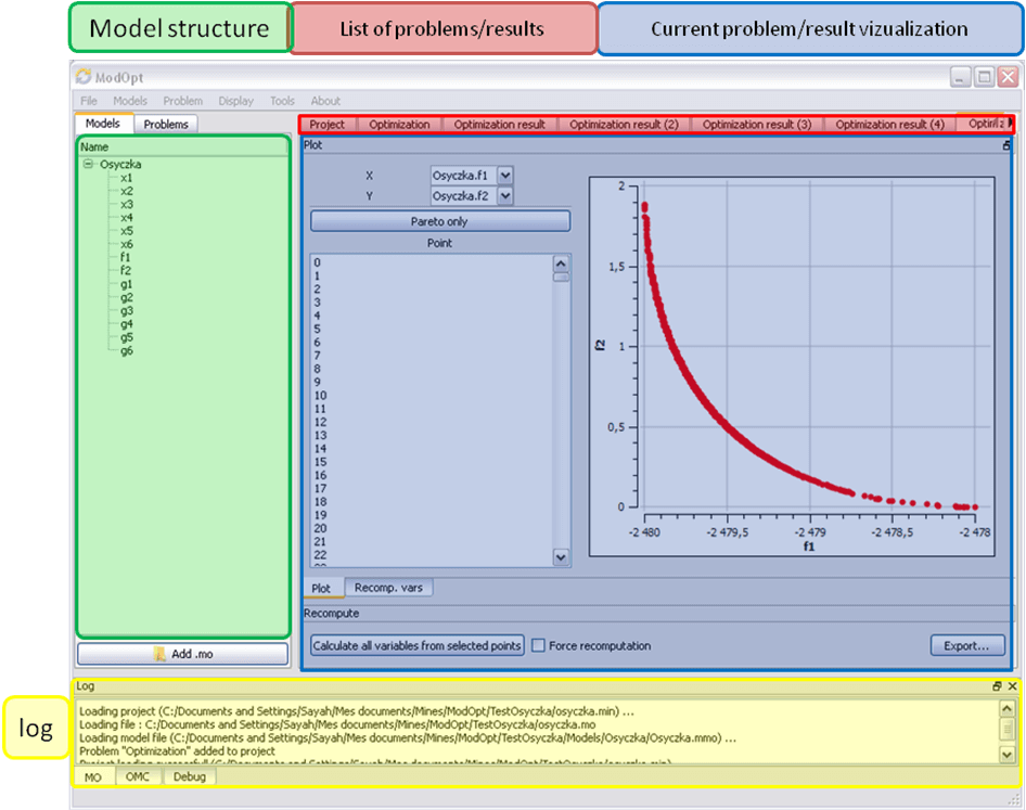
Figure 66 Window regions in OMOptim GUI.

[BOR+12]

Bernhard Bachmann, Lennart Ochel, Vitalij Ruge, Mahder Gebremedhin, Peter Fritzson, Vaheed Nezhadali, Lars Eriksson, and Martin Sivertsson. Parallel multiple-shooting and collocation Optimization with OpenModelica. In Martin Otter and Dirk Zimmer, editors, Proceedings of the 9th International Modelica Conference. Linköping University Electronic Press, sep 2012. doi:10.3384/ecp12076659.

[RBB+14]

Vitalij Ruge, Willi Braun, Bernhard Bachmann, Andrea Walther, and Kshitij Kulshreshtha. Efficient implementation of collocation methods for optimization using openmodelica and adol-c. In Hubertus Tummescheit and Karl-Erik Årzén, editors, Proceedings of the 10th International Modelica Conference. Modelica Association and Linköping University Electronic Press, mar 2014. doi:10.3384/ecp140961017.