OMNotebook with DrModelica and DrControl
This chapter covers the OpenModelica electronic notebook subsystem, called OMNotebook, together with the DrModelica tutoring system for teaching Modelica, and DrControl for teaching control together with Modelica. Both are using such notebooks.
Interactive Notebooks with Literate Programming
Interactive Electronic Notebooks are active documents that may contain technical computations and text, as well as graphics. Hence, these documents are suitable to be used for teaching and experimentation, simulation scripting, model documentation and storage, etc.
Mathematica Notebooks
Literate Programming [Knu84] is a form of programming where programs are integrated with documentation in the same document. Mathematica notebooks [Wol96] is one of the first WYSIWYG systems that support Literate Programming. Such notebooks are used, e.g., in the MathModelica modeling and simulation environment, see e.g. Figure 49 below and Chapter 19 in [Fri04].
OMNotebook
The OMNotebook software [Axe05][Fernstrom06] is a new open source free software that gives an interactive WYSIWYG realization of Literate Programming, a form of programming where programs are integrated with documentation in the same document.
The OMNotebook facility is actually an interactive WYSIWYG realization of Literate Programming, a form of programming where programs are integrated with documentation in the same document. OMNotebook is a simple open-source software tool for an electronic notebook supporting Modelica.
A more advanced electronic notebook tool, also supporting mathematical typesetting and many other facilities, is provided by Mathematica notebooks in the MathModelica environment, see Figure 49.
Figure 49 Examples of Mathematica notebooks in the MathModelica modeling and simulation environment.
Traditional documents, e.g. books and reports, essentially always have a hierarchical structure. They are divided into sections, subsections, paragraphs, etc. Both the document itself and its sections usually have headings as labels for easier navigation. This kind of structure is also reflected in electronic notebooks. Every notebook corresponds to one document (one file) and contains a tree structure of cells. A cell can have different kinds of contents, and can even contain other cells. The notebook hierarchy of cells thus reflects the hierarchy of sections and subsections in a traditional document such as a book.
DrModelica Tutoring System – an Application of OMNotebook
Understanding programs is hard, especially code written by someone else. For educational purposes it is essential to be able to show the source code and to give an explanation of it at the same time.
Moreover, it is important to show the result of the source code’s execution. In modeling and simulation it is also important to have the source code, the documentation about the source code, the execution results of the simulation model, and the documentation of the simulation results in the same document. The reason is that the problem solving process in computational simulation is an iterative process that often requires a modification of the original mathematical model and its software implementation after the interpretation and validation of the computed results corresponding to an initial model.
Most of the environments associated with equation-based modeling languages focus more on providing efficient numerical algorithms rather than giving attention to the aspects that should facilitate the learning and teaching of the language. There is a need for an environment facilitating the learning and understanding of Modelica. These are the reasons for developing the DrModelica teaching material for Modelica and for teaching modeling and simulation.
An earlier version of DrModelica was developed using the MathModelica (now Wolfram SystemModeler) environment. The rest of this chapter is concerned with the OMNotebook version of DrModelica and on the OMNotebook tool itself.
DrModelica has a hierarchical structure represented as notebooks. The front-page notebook is similar to a table of contents that holds all other notebooks together by providing links to them. This particular notebook is the first page the user will see (Figure 50).
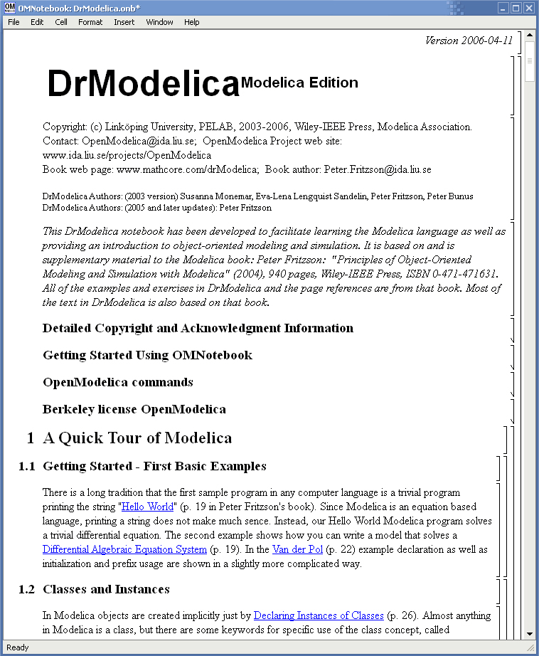
Figure 50 The front-page notebook of the OMNotebook version of the DrModelica tutoring system.
In each chapter of DrModelica the user is presented a short summary of the corresponding chapter of the Modelica book [Fri04]. The summary introduces some keywords, being hyperlinks that will lead the user to other notebooks describing the keywords in detail.
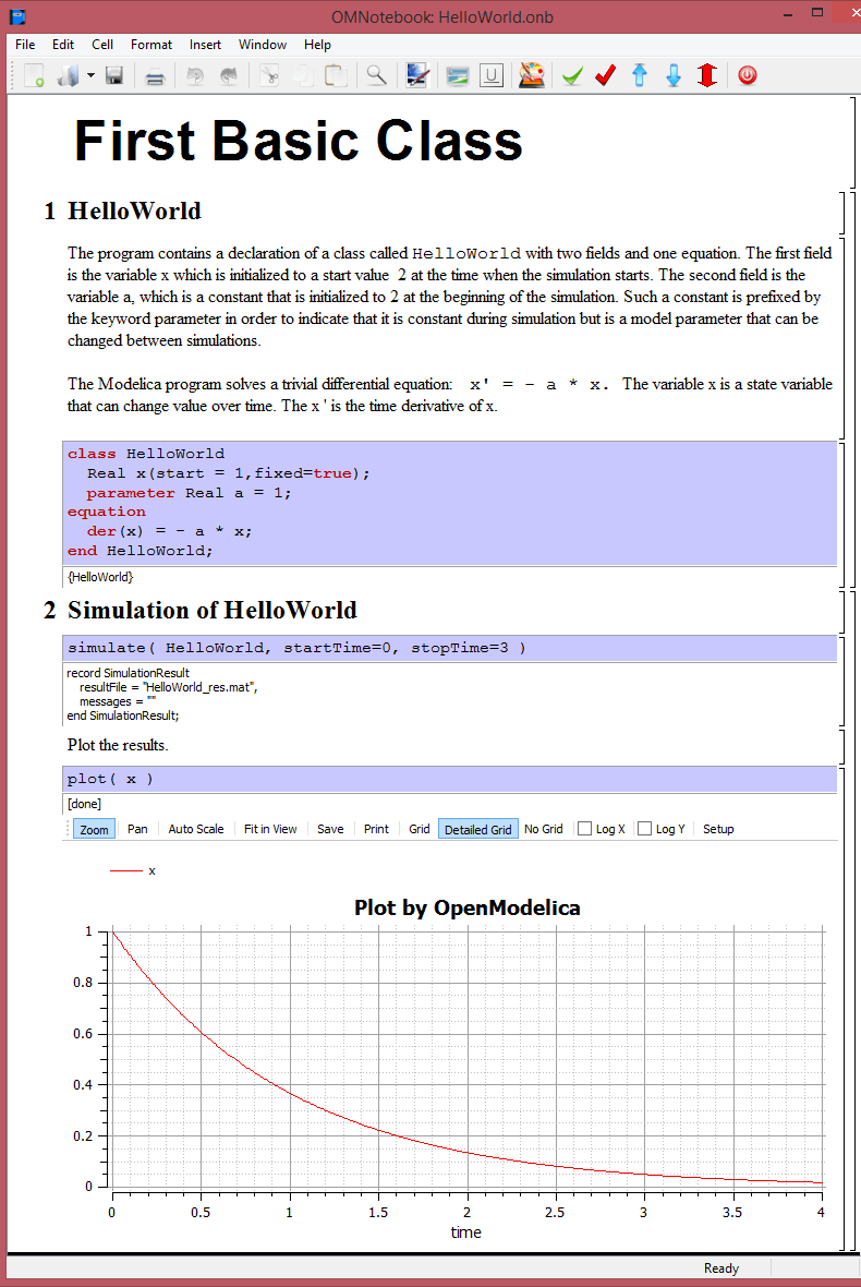
Figure 51 The HelloWorld class simulated and plotted using the OMNotebook version of DrModelica.
Now, let us consider that the link “HelloWorld” in DrModelica Section is clicked by the user. The new HelloWorld notebook (see Figure 51), to which the user is being linked, is not only a textual description but also contains one or more examples explaining the specific keyword. In this class, HelloWorld, a differential equation is specified.
No information in a notebook is fixed, which implies that the user can add, change, or remove anything in a notebook. Alternatively, the user can create an entirely new notebook in order to write his/her own programs or copy examples from other notebooks. This new notebook can be linked from existing notebooks.
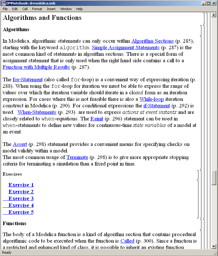
Figure 52 DrModelica Chapter on Algorithms and Functions in the main page of the OMNotebook version of DrModelica.
When a class has been successfully evaluated the user can simulate and plot the result, as previously depicted in Figure 51 for the simple HelloWorld example model.
After reading a chapter in DrModelica the user can immediately practice the newly acquired information by doing the exercises that concern the specific chapter. Exercises have been written in order to elucidate language constructs step by step based on the pedagogical assumption that a student learns better “using the strategy of learning by doing”. The exercises consist of either theoretical questions or practical programming assignments. All exercises provide answers in order to give the user immediate feedback.
Figure 52 shows part of Chapter 9 of the DrModelica teaching material. Here the user can read about language constructs, like algorithm sections, when-statements, and reinit equations, and then practice these constructs by solving the exercises corresponding to the recently studied section.
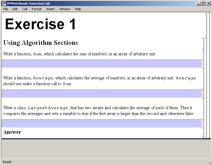
Figure 53 Exercise 1 in Chapter 9 of DrModelica.
Exercise 1 from Chapter 9 is shown in Figure 53. In this exercise the user has the opportunity to practice different language constructs and then compare the solution to the answer for the exercise. Notice that the answer is not visible until the Answer section is expanded. The answer is shown in Figure 54.
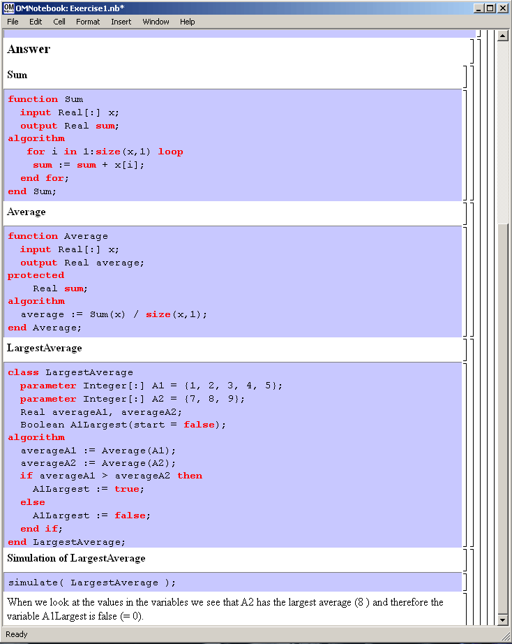
Figure 54 The answer section to Exercise 1 in Chapter 9 of DrModelica.
DrControl Tutorial for Teaching Control Theory
DrControl is an interactive OMNotebook document aimed at teaching control theory. It is included in the OpenModelica distribution and appears under the directory:
>>> getInstallationDirectoryPath() + "/share/omnotebook/drcontrol"
"«OPENMODELICAHOME»/share/omnotebook/drcontrol"
The front-page of DrControl resembles a linked table of content that can be used as a navigation center. The content list contains topics like:
- Getting started
- The control problem in ordinary life
- Feedback loop
- Mathematical modeling
- Transfer function
- Stability
- Example of controlling a DC-motor
- Feedforward compensation
- State-space form
- State observation
- Closed loop control system.
- Reconstructed system
- Linear quadratic optimization
- Linearization
Each entry in this list leads to a new notebook page where either the theory is explained with Modelica examples or an exercise with a solution is provided to illustrate the background theory. Below we show a few sections of DrControl.
Feedback Loop
One of the basic concepts of control theory is using feedback loops either for neutralizing the disturbances from the surroundings or a desire for a smoother output.
In Figure 55, control of a simple car model is illustrated where the car velocity on a road is controlled, first with an open loop control, and then compared to a closed loop system with a feedback loop. The car has a mass m, velocity y, and aerodynamic coefficient α. The θ is the road slope, which in this case can be regarded as noise.
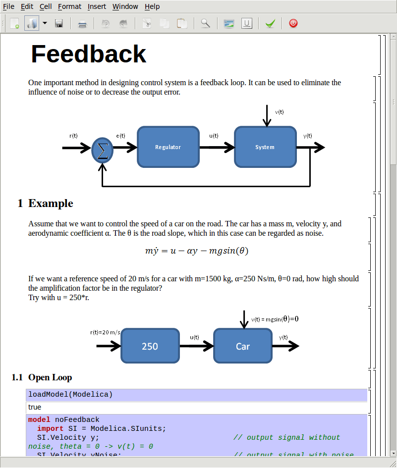
Figure 55 Feedback loop.
Lets look at the Modelica model for the open loop controlled car:
model noFeedback
  import SI = Modelica.SIunits;
  SI.Velocity y;                              // output signal without noise, theta = 0 -> v(t) = 0
  SI.Velocity yNoise;                         // output signal with noise,    theta <> 0 -> v(t) <> 0
  parameter SI.Mass m = 1500;
  parameter Real alpha = 200;
  parameter SI.Angle theta = 5*3.141592/180;
  parameter SI.Acceleration g = 9.82;
  SI.Force u;
  SI.Velocity r=20;
equation
  m*der(y)=u-alpha*y;                          // signal without noise
  m*der(yNoise)=u-alpha*yNoise-m*g*sin(theta); // with noise
  u = 250*r;
end noFeedback;
By applying a road slope angle different from zero the car velocity is influenced which can be regarded as noise in this model. The output signal in Figure 56 is stable but an overshoot can be observed compared to the reference signal. Naturally the overshoot is not desired and the student will in the next exercise learn how to get rid of this undesired behavior of the system.
>>> loadModel(Modelica)
true
>>> simulate(noFeedback, stopTime=100)
record SimulationResult
    resultFile = "«DOCHOME»/noFeedback_res.mat",
    simulationOptions = "startTime = 0.0, stopTime = 100.0, numberOfIntervals = 500, tolerance = 1e-06, method = 'dassl', fileNamePrefix = 'noFeedback', options = '', outputFormat = 'mat', variableFilter = '.*', cflags = '', simflags = ''",
    messages = "LOG_SUCCESS       | info    | The initialization finished successfully without homotopy method.
LOG_SUCCESS       | info    | The simulation finished successfully.
",
    timeFrontend = 0.251943035,
    timeBackend = 0.005860424,
    timeSimCode = 0.161887682,
    timeTemplates = 0.100463247,
    timeCompile = 0.6459081800000001,
    timeSimulation = 0.008208341000000001,
    timeTotal = 1.174420463
end SimulationResult;
Warning
Warning: The initial conditions are not fully specified. For more information set -d=initialization. In OMEdit Tools->Options->Simulation->OMCFlags, in OMNotebook call setCommandLineOptions("-d=initialization").
Figure 56 Open loop control example.
The closed car model with a proportional regulator is shown below:
model withFeedback
  import SI = Modelica.SIunits;
  SI.Velocity y;                                // output signal with feedback link and without noise, theta = 0 -> v(t) = 0
  SI.Velocity yNoise;                           // output signal with feedback link and noise,    theta <> 0 -> v(t) <> 0
  parameter SI.Mass m = 1500;
  parameter Real alpha = 250;
  parameter SI.Angle theta = 5*3.141592/180;
  parameter SI.Acceleration g = 9.82;
  SI.Force u;
  SI.Force uNoise;
  SI.Velocity r=20;
equation
  m*der(y)=u-alpha*y;
  m*der(yNoise)=uNoise-alpha*yNoise-m*g*sin(theta);
  u = 5000*(r-y);
  uNoise = 5000*(r-yNoise);
end withFeedback;
By using the information about the current level of the output signal and re-tune the regulator the output quantity can be controlled towards the reference signal smoothly and without an overshoot, as shown in Figure 57.
In the above simple example the flat modeling approach was adopted since it was the fastest one to quickly obtain a working model. However, one could use the object oriented approach and encapsulate the car and regulator models in separate classes with the Modelica connector mechanism in between.
>>> loadModel(Modelica)
true
>>> simulate(withFeedback, stopTime=10)
record SimulationResult
    resultFile = "«DOCHOME»/withFeedback_res.mat",
    simulationOptions = "startTime = 0.0, stopTime = 10.0, numberOfIntervals = 500, tolerance = 1e-06, method = 'dassl', fileNamePrefix = 'withFeedback', options = '', outputFormat = 'mat', variableFilter = '.*', cflags = '', simflags = ''",
    messages = "LOG_SUCCESS       | info    | The initialization finished successfully without homotopy method.
LOG_SUCCESS       | info    | The simulation finished successfully.
",
    timeFrontend = 0.373659364,
    timeBackend = 0.004083695,
    timeSimCode = 0.2017354889999999,
    timeTemplates = 0.08356058000000001,
    timeCompile = 0.653635478,
    timeSimulation = 0.008507468000000001,
    timeTotal = 1.325323178
end SimulationResult;
Warning
Warning: The initial conditions are not fully specified. For more information set -d=initialization. In OMEdit Tools->Options->Simulation->OMCFlags, in OMNotebook call setCommandLineOptions("-d=initialization").
Figure 57 Closed loop control example.
Mathematical Modeling with Characteristic Equations
In most systems the relation between the inputs and outputs can be described by a linear differential equation. Tearing apart the solution of the differential equation into homogenous and particular parts is an important technique taught to the students in engineering courses, also illustrated in Figure 58.
Now let us examine a second order system:
model NegRoots
  Real y;
  Real der_y;
  parameter Real a1 = 3;
  parameter Real a2 = 2;
equation
  der_y = der(y);
  der(der_y) + a1*der_y + a2*y = 1;
end NegRoots;
Choosing different values for a1 and a2 leads to different behavior as shown in Figure 59 and Figure 60.
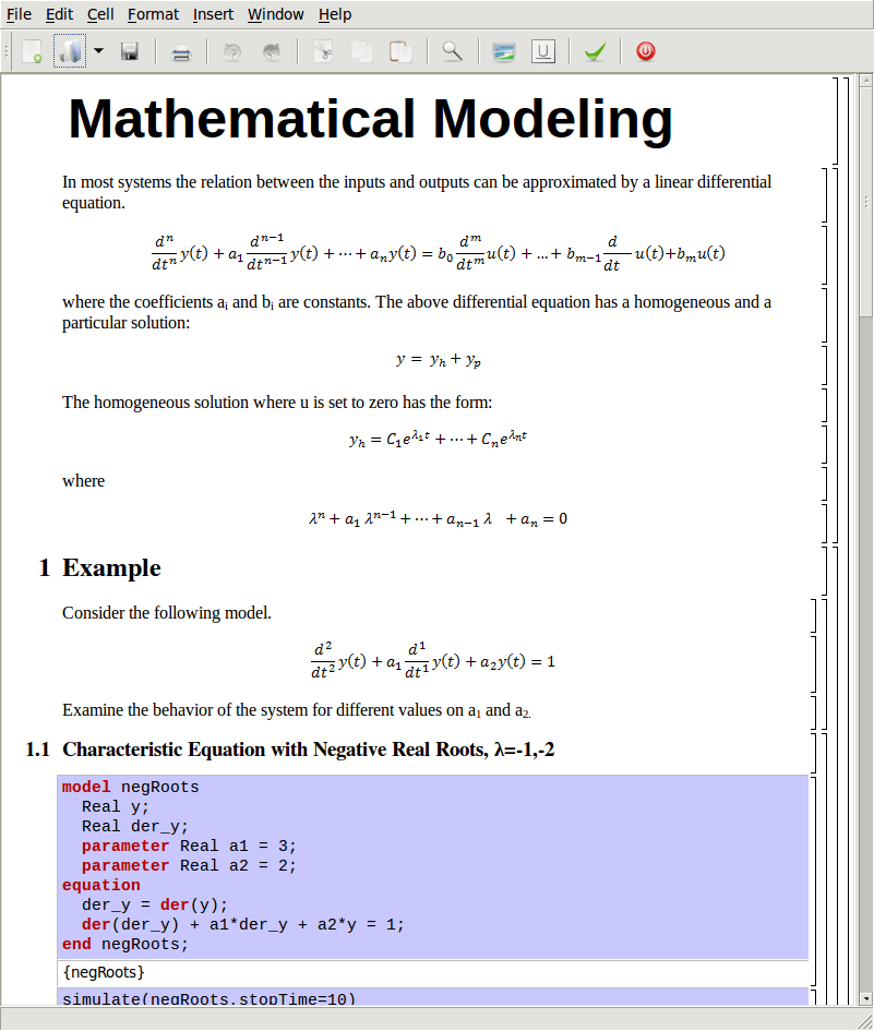
Figure 58 Mathematical modeling with characteristic equation.
In the first example the values of a1 and a2 are chosen in such way that the characteristic equation has negative real roots and thereby a stable output response, see Figure 59.
>>> simulate(NegRoots, stopTime=10)
record SimulationResult
    resultFile = "«DOCHOME»/NegRoots_res.mat",
    simulationOptions = "startTime = 0.0, stopTime = 10.0, numberOfIntervals = 500, tolerance = 1e-06, method = 'dassl', fileNamePrefix = 'NegRoots', options = '', outputFormat = 'mat', variableFilter = '.*', cflags = '', simflags = ''",
    messages = "LOG_SUCCESS       | info    | The initialization finished successfully without homotopy method.
LOG_SUCCESS       | info    | The simulation finished successfully.
",
    timeFrontend = 0.4506635530000001,
    timeBackend = 0.002796812,
    timeSimCode = 0.185741627,
    timeTemplates = 0.118964785,
    timeCompile = 0.6573220019999999,
    timeSimulation = 0.008306504000000001,
    timeTotal = 1.423938817
end SimulationResult;
Warning
Warning: The initial conditions are not fully specified. For more information set -d=initialization. In OMEdit Tools->Options->Simulation->OMCFlags, in OMNotebook call setCommandLineOptions("-d=initialization").
Figure 59 Characteristic equation with real negative roots.
The importance of the sign of the roots in the characteristic equation is illustrated in Figure 59 and Figure 60, e.g., a stable system with negative real roots and an unstable system with positive imaginary roots resulting in oscillations.
model ImgPosRoots
  Real y;
  Real der_y;
  parameter Real a1 = -2;
  parameter Real a2 = 10;
equation
  der_y = der(y);
  der(der_y) + a1*der_y + a2*y = 1;
end ImgPosRoots;
>>> simulate(ImgPosRoots, stopTime=10)
record SimulationResult
    resultFile = "«DOCHOME»/ImgPosRoots_res.mat",
    simulationOptions = "startTime = 0.0, stopTime = 10.0, numberOfIntervals = 500, tolerance = 1e-06, method = 'dassl', fileNamePrefix = 'ImgPosRoots', options = '', outputFormat = 'mat', variableFilter = '.*', cflags = '', simflags = ''",
    messages = "LOG_SUCCESS       | info    | The initialization finished successfully without homotopy method.
LOG_SUCCESS       | info    | The simulation finished successfully.
",
    timeFrontend = 0.210849718,
    timeBackend = 0.002496992,
    timeSimCode = 0.151999258,
    timeTemplates = 0.09730607399999991,
    timeCompile = 0.630074052,
    timeSimulation = 0.00823607,
    timeTotal = 1.101086089
end SimulationResult;
Warning
Warning: The initial conditions are not fully specified. For more information set -d=initialization. In OMEdit Tools->Options->Simulation->OMCFlags, in OMNotebook call setCommandLineOptions("-d=initialization").
Figure 60 Characteristic equation with imaginary roots with positive real part.
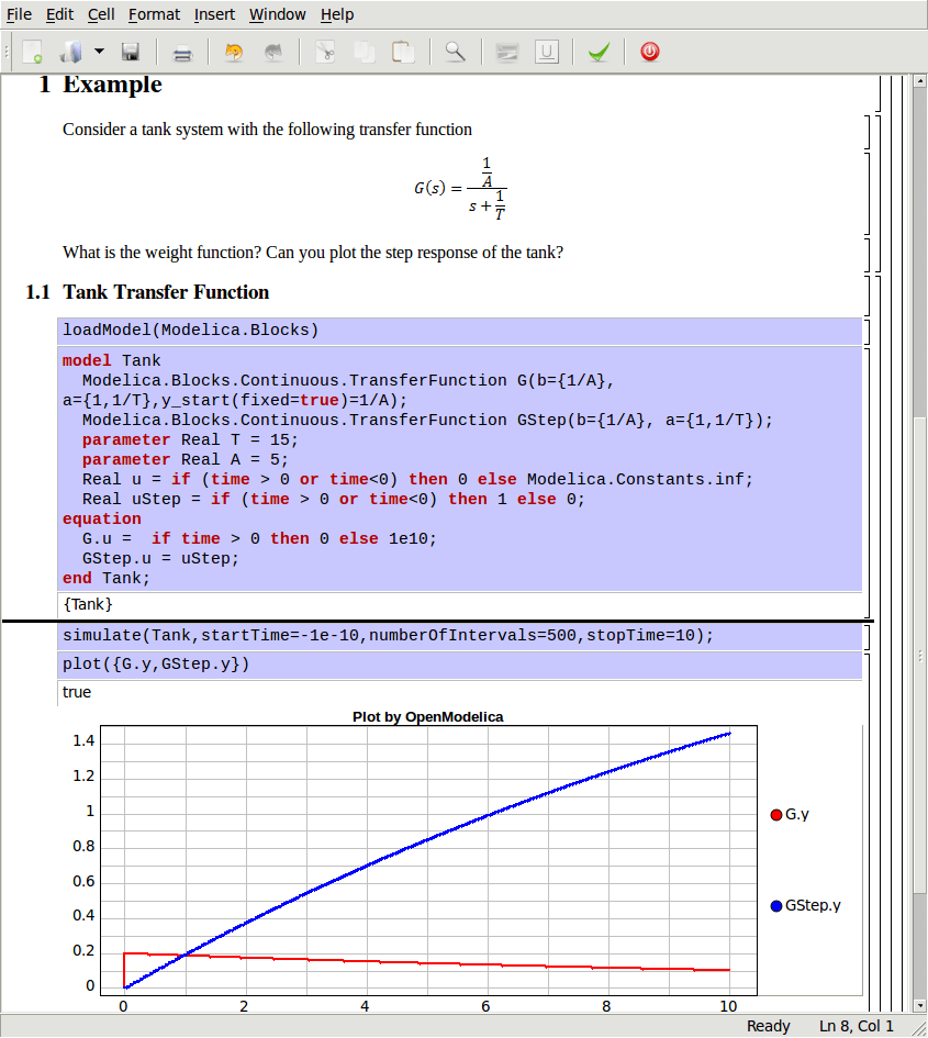
Figure 61 Step and pulse (weight function) response.
The theory and application of Kalman filters is also explained in the interactive course material.
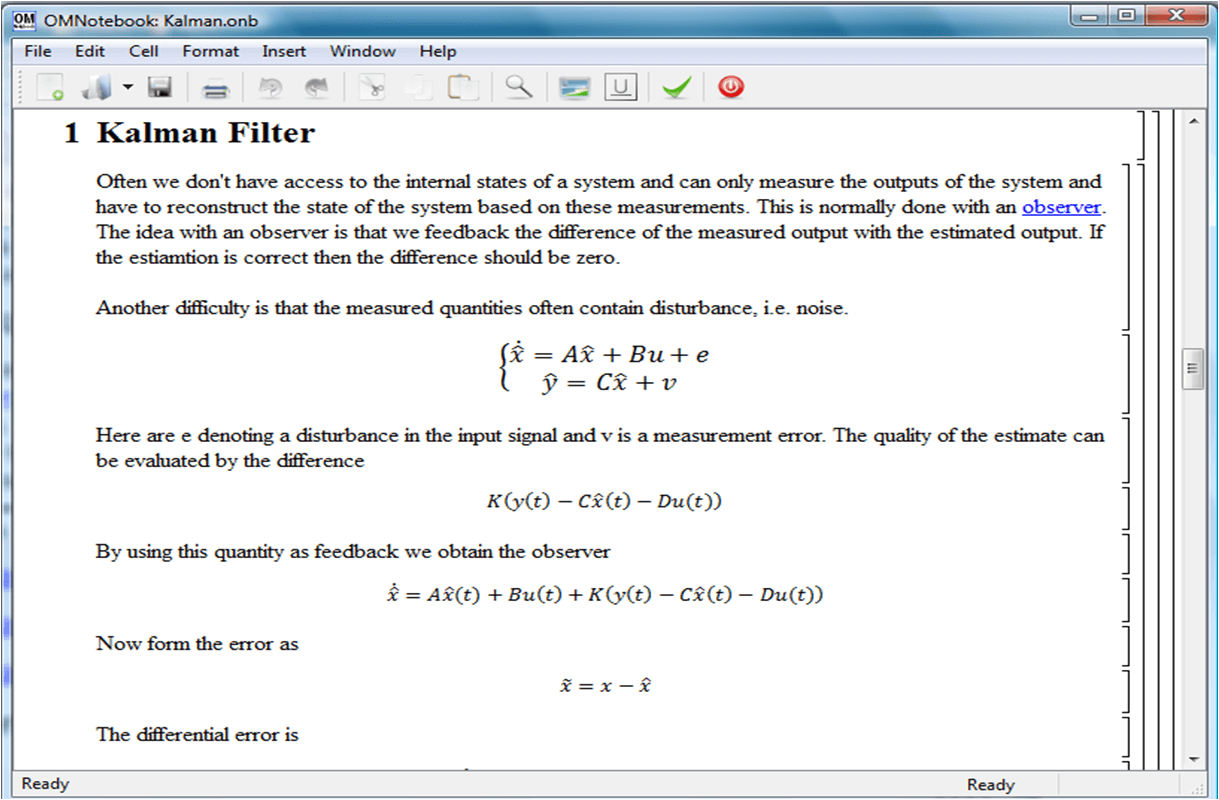
Figure 62 Theory background about Kalman filter.
In reality noise is present in almost every physical system under study and therefore the concept of noise is also introduced in the course material, which is purely Modelica based.
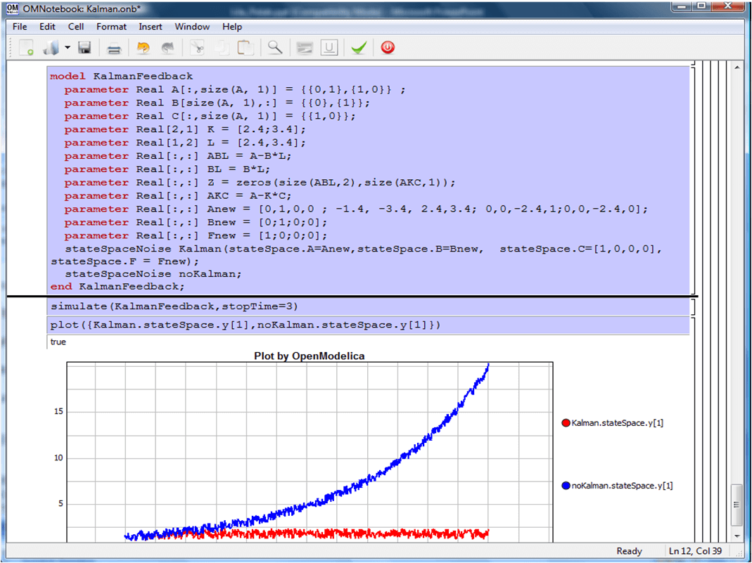
Figure 63 Comparison of a noisy system with feedback link in DrControl.
OpenModelica Notebook Commands
OMNotebook currently supports the commands and concepts that are described in this section.
Cells
Everything inside an OMNotebook document is made out of cells. A cell basically contains a chunk of data. That data can be text, images, or other cells. OMNotebook has four types of cells: headercell, textcell, inputcell, and groupcell. Cells are ordered in a tree structure, where one cell can be a parent to one or more additional cells. A tree view is available close to the right border in the notebook window to display the relation between the cells.
- Textcell – This cell type is used to display ordinary text and
- images. Each textcell has a style that specifies how text is displayed. The cell´s style can be changed in the menu Format->Styles, example of different styles are: Text, Title, and Subtitle. The Textcell type also has support for following links to other notebook documents.
- Inputcell – This cell type has support for syntax highlighting and
- evaluation. It is intended to be used for writing program code, e.g. Modelica code. Evaluation is done by pressing the key combination Shift+Return or Shift+Enter. All the text in the cell is sent to OMC (OpenModelica Compiler/interpreter), where the text is evaluated and the result is displayed below the inputcell. By double-clicking on the cell marker in the tree view, the inputcell can be collapsed causing the result to be hidden.
- Latexcell – This cell type has support for evaluation of latex scripts.
- It is intended to be mainly used for writing mathematical equations and formulas for advanced documentation in OMNotebook. Each Latexcell supports a maximum of one page document output.To evaluate this cell, latex must be installed in your system.The users can copy and paste the latex scripts and start the evaluation.Evaluation is done by pressing the key combination Shift+Return or Shift+Enter or the green color eval button present in the toolbar. The script in the cell is sent to latex compiler, where it is evaluated and the output is displayed hiding the latex source. By double-clicking on the cell marker in the tree view,the latex source is displayed for further modification.
- Groupcell – This cell type is used to group together other cell. A
- groupcell can be opened or closed. When a groupcell is opened all the cells inside the groupcell are visible, but when the groupcell is closed only the first cell inside the groupcell is visible. The state of the groupcell is changed by the user double-clicking on the cell marker in the tree view. When the groupcell is closed the marker is changed and the marker has an arrow at the bottom.
Cursors
An OMNotebook document contains cells which in turn contain text. Thus, two kinds of cursors are needed for positioning, text cursor and cell cursor:
- Textcursor – A cursor between characters in a cell, appearing as a
- small vertical line. Position the cursor by clicking on the text or using the arrow buttons.
- Cellcursor – This cursor shows which cell currently has the input
- focus. It consists of two parts. The main cellcursor is basically just a thin black horizontal line below the cell with input focus. The cellcursor is positioned by clicking on a cell, clicking between cells, or using the menu item Cell->Next Cell or Cell->Previous Cell. The cursor can also be moved with the key combination Ctrl+Up or Ctrl+Down. The dynamic cellcursor is a short blinking horizontal line. To make this visible, you must click once more on the main cellcursor (the long horizontal line). NOTE: In order to paste cells at the cellcursor, the dynamic cellcursor must be made active by clicking on the main cellcursor (the horizontal line).
Selection of Text or Cells
To perform operations on text or cells we often need to select a range of characters or cells.
- Select characters – There are several ways of selecting characters,
- e.g. double-clicking on a word, clicking and dragging the mouse, or click followed by a shift-click at an adjacent positioin selects the text between the previous click and the position of the most recent shift-click.
- Select cells – Cells can be selected by clicking on them. Holding
- down Ctrl and clicking on the cell markers in the tree view allows several cells to be selected, one at a time. Several cells can be selected at once in the tree view by holding down the Shift key. Holding down Shift selects all cells between last selected cell and the cell clicked on. This only works if both cells belong to the same groupcell.
Additional Features
- Links – By clicking on a link, OMNotebook will open the document
- that is referred to in the link.
- Update link – All links are stored with relative file path.
- Therefore OMNotebook has functions that automatically updating links if a document is resaved in another folder. Every time a document is saved, OMNotebook checks if the document is saved in the same folder as last time. If the folder has changed, the links are updated.
- Evaluate whole Notebook – All the cells present in the Notebook can
- be evaluated in one step by pressing the red color evalall button in the toolbar. The cells are evaluated in the same order as they are in the Notebook.However the latexcells cannot be evaluated by this feature.
- Evaluate several cells – Several inputcells can be evaluated at
- the same time by selecting them in the treeview and then pressing the key combination Shift+Enter or Shift+Return. The cells are evaluated in the same order as they have been selected. If a groupcell is selected all inputcells in that groupcell are evaluated, in the order they are located in the groupcell.
- Moving and Reordering cells in a Notebook – It is possible to shift cells
- to a new position and change the hierarchical order of the document.This can be done by clicking the cell and press the Up and Down arrow button in the tool bar to move either Up or Down. The cells are moved one cell above or below.It is also possible to move a cell directly to a new position with one single click by pressing the red color bidirectional UpDown arrow button in the toolbar. To do this the user has to place the cell cursor to a position where the selected cells must be moved. After selecting the cell cursor position, select the cells you want to shift and press the bidirectional UpDown arrow button. The cells are shifted in the same order as they are selected.This is especially very useful when shifting a group cell.
- Command completion – Inputcells have command completion support,
- which checks if the user is typing a command (or any keyword defined in the file commands.xml) and finish the command. If the user types the first two or three letters in a command, the command completion function fills in the rest. To use command completion, press the key combination Ctrl+Space or Shift+Tab. The first command that matches the letters written will then appear. Holding down Shift and pressing Tab (alternative holding down Ctrl and pressing Space) again will display the second command that matches. Repeated request to use command completion will loop through all commands that match the letters written. When a command is displayed by the command completion functionality any field inside the command that should be edited by the user is automatically selected. Some commands can have several of these fields and by pressing the key combination Ctrl+Tab, the next field will be selected inside the command. > Active Command completion: Ctrl+Space / Shift+Tab > Next command: Ctrl+Space / Shift+Tab > Next field in command: Ctrl+Tab’
- Generated plot – When plotting a simulation result, OMC uses the
- program Ptplot to create a plot. From Ptplot OMNotebook gets an image of the plot and automatically adds that image to the output part of an inputcell. Like all other images in a document, the plot is saved in the document file when the document is saved.
- Stylesheet –OMNotebook follows the style settings defined in
- stylesheet.xml and the correct style is applied to a cell when the cell is created.
- Automatic Chapter Numbering – OMNotebook automatically numbers
- different chapter, subchapter, section and other styles. The user can specify which styles should have chapter numbers and which level the style should have. This is done in the stylesheet.xml file. Every style can have a <chapterLevel> tag that specifies the chapter level. Level 0 or no tag at all, means that the style should not have any chapter numbering.
- Scrollarea – Scrolling through a document can be done by using the
- mouse wheel. A document can also be scrolled by moving the cell cursor up or down.
- Syntax highlighter – The syntax highlighter runs in a separated
- thread which speeds up the loading of large document that contains many Modelica code cells. The syntax highlighter only highlights when letters are added, not when they are removed. The color settings for the different types of keywords are stored in the file modelicacolors.xml. Besides defining the text color and background color of keywords, whether or not the keywords should be bold or/and italic can be defined.
- Change indicator – A star (*) will appear behind the filename in
- the title of notebook window if the document has been changed and needs saving. When the user closes a document that has some unsaved change, OMNotebook asks the user if he/she wants to save the document before closing. If the document never has been saved before, the save-as dialog appears so that a filename can be choosen for the new document.
- Update menus – All menus are constantly updated so that only menu
- items that are linked to actions that can be performed on the currently selected cell is enabled. All other menu items will be disabled. When a textcell is selected the Format menu is updated so that it indicates the text settings for the text, in the current cursor position.
References
Todo
Add these into extrarefs.bib and cite them somewhere
Eric Allen, Robert Cartwright, Brian Stoler. DrJava: A lightweight pedagogic environment for Java. In Proceedings of the 33rd ACM Technical Symposium on Computer Science Education (SIGCSE 2002) (Northern Kentucky – The Southern Side of Cincinnati, USA, February 27 – March 3, 2002).
Anders Fernström, Ingemar Axelsson, Peter Fritzson, Anders Sandholm, Adrian Pop. OMNotebook – Interactive WYSIWYG Book Software for Teaching Programming. In Proc. of the Workshop on Developing Computer Science Education – How Can It Be Done?. Linköping University, Dept. Computer & Inf. Science, Linköping, Sweden, March 10, 2006.
Eva-Lena Lengquist-Sandelin, Susanna Monemar, Peter Fritzson, and Peter Bunus. DrModelica – A Web-Based Teaching Environment for Modelica. In Proceedings of the 44th Scandinavian Conference on Simulation and Modeling (SIMS’2003), available at www.scan-sims.org. Västerås, Sweden. September 18-19, 2003.
| [Axe05] | Ingemar Axelsson. OpenModelica Notebook for interactive structured Modelica documents. Master's thesis, Linköping University, Department of Computer and Information Science, October 2005. LITH-IDA-EX–05/080–SE. |
| [Fernstrom06] | Anders Fernström. Extending OpenModelica Notebook – an interactive notebook for structured Modelica documents. Master's thesis, Linköping University, Department of Computer and Information Science, September 2006. LITH-IDA-EX–06/057—SE. |
| [Fri04] | (1, 2) Peter Fritzson. Principles of Object-Oriented Modeling and Simulation with Modelica 2.1. Wiley-IEEE Press, February 2004. ISBN 0-471-471631. |
| [Knu84] | Donald E. Knuth. Literate programming. The Computer Journal, 27:97–111, 1984. |
| [Wol96] | Stephen Wolfram. The Mathematica Book. Wolfram Media/Cambridge University Press, third edition, 1996. |