Optimization with OpenModelica¶

The following facilities for model-based optimization are provided with OpenModelica:

Built-in Dynamic Optimization using Annotations using dynamic optimization is the recommended way of performing dynamic optimization with OpenModelica.
Dynamic Optimization with OpenModelica and CasADi. Use this if you want to employ the CasADi tool for dynamic optimization.
Classical Parameter Sweep Optimization using OMOptim. Use this if you have a static optimization problem.

Built-in Dynamic Optimization using Annotations¶

This part of the OM manual is a contribution by Massimo Ceraolo and Vitalij Ruge.

Foreword¶

Dynamic optimization using Annotations is the most user-friendly way to perform Dynamic Optimization(DO) in OpenModelica, since it allows the OMEdit graphical user interface to be used.

It is also more powerful that the Built-in Dynamic Optimization using Optimica language extensions, since it allows final constraints.

Formulation limitations and algorithm¶

We can formulate the optimization problem as follows:

$\begin{eqnarray} \min_{u(t)}{\ \left\lbrack M\left( \mathbf{x}\left( t_{f} \right), \mathbf{u}\left( t_{f} \right),t_{f} \right) + \int_{t_{0}}^{t_{f}}{L\left( \mathbf{x}(t), \mathbf{u}(t),t \right)\text{dt}} \right\rbrack} && \begin{array}[t]{l} \mbox{optimization purpose} \\ (M \mbox{ \textit{is the Mayer Term}} \\ L \mbox{ \textit{is the Lagrange Term}}) \end{array} \\ \mathbf{0} = \mathbf{f}\left( \mathbf{x}(t),\dot{\mathbf{x}}(t),\mathbf{u}(t),t \right) && \begin{array}[t]{l} \mbox{dynamical description} \\ \mbox{of the system} \end{array} \\ \mathbf{0} \leq \mathbf{g}\left( \mathbf{x}(t),\mathbf{u}(t),t \right) && \begin{array}[t]{l} \mbox{path constraints} \\ \mbox{e.g. physical limits of components} \end{array} \\ \mathbf{0} = \mathbf{r}_{0}\left( \mathbf{x}\left(t_{0} \right),t_{0} \right) && \mbox{Initial constraint} \\ \mathbf{0} = \mathbf{r}_{f}(\mathbf{x}\left( t_{f} \right)\mathbf{u}\left( t_{f} \right),t_{f}) && \mbox{Final constraint} \end{eqnarray}$

Where u(t) is the vector of input variables, on which DO works to try to get the desired minimum, and x(t) is the vector of state variables.

The equations above can be implemented in OpenModelica using the full power of Modelica language, and therefore there is a good freedom and flexibility, under the obvious constraint that the system must be regular enough for the convergence to take place.

However, there are limitations in the possibility operational limits can be set.

The formulation of operational limits in (3) is general, since it allows to use non-boxed constrains. Consider for instance a battery. The energy the battery can deliver is a function of the power we use to charge or discharge it. Therefore, the actual limit should be described as:

$E_{\min}(P) \leq E_{\text{bat}} \leq E_{\max}(P)$

Moreover, (3) is time-variant (the third argument of function g).

The OpenModelica optimization through annotations accepts as path constraints only time-invariant box constraints, so eq (3) is expressed in the simpler form:

$\mathbf{x}_{\min} \leq \mathbf{x}(t) \leq \mathbf{x}_{\max}$

$\mathbf{u}_{\min} \leq \mathbf{u}(t) \leq \mathbf{u}_{\max}$

$g_{\min} \leq g(\mathbf{x}(t),\mathbf{u}(t)) \leq g_{\max}$

OpenModelica uses the Radau IIA discretization scheme of order 1 or 5 depending on user input.

Using the first order the Radau IIA is equivalent to implicit Euler and to compute states, output and cost function only the values at the end of each interval are evaluated. E.g., if we have StopTime=1 and Interval=0.25, only values for t=0.25, t=0.5, t=0.75, t=1 will be considered. Therefore, the resulting value of the control variable at t=0 may be even totally wrong, since it has no influence on the result.

Syntax¶

OpenModelica provides specific annotations to allow the optimization problem to be described, as an alternative to the use of Optimica language. They are listed and commented below.

Request for an optimization. We must use two simulation flags and a command line option. These can conveniently be inserted into the code, to avoid selecting them manually all the time, as follows:
```
__OpenModelica_simulationFlags(s = "optimization", optimizerNP="1"),
__OpenModelica_commandLineOptions = "+g=Optimica",
```
OptimizerNP gives the number of colloction points and can be only 1 or 3. As already said the RadauIIA order is 2*OptimizerNP-1.

The user is recommended to use as a first attempt optimizerNP=1. In case of questionable results, they can try optimizerNP=3.

For the simulation, it is known that the stability ranges are different. At the same time, we lose stability with higher order (see [1]).

Note that Optimica command-line option is added even if we do not use Optimica specific language constructs; this it is required for the use of optimization-related annotations.
Select optimization parameters. We must specify StartTime, StopTime, Interval, and Tolerance. The first two have the same meaning as in time simulations. Interval not only defines the output interval (as in time simulations), but has a more specific meaning: it defines the interval between two successive collocation points. I.e., optimization is done splitting the whole timespan in sparts having interval as length. Therefore this value may have a huge effects on the simulation output. For typical runs, number of intervals values from 100 to 1000-2000 could be adequate. These values are obviously set through the experiment annotation, e.g.:
```
experiment(StartTime = 0, StopTime = 20, Tolerance = 1e-07, Interval = 0.02),
```
the default tolerance is 1e-6. The user is warned that enlarging this value may affect the output quality adversely by large amounts (an example will be provided later). Going up to 1e-8 may be advisable in some cases.
Define the variable(s) to be determined by DO. The variables the DO must determine must have the input attribute. They can have (with parameter variability) min and max attributes, which are interpreted as boxed path constraints on input. It is recommended to also define a start value for them, since it is used for initialization (see sect. DO Initialization). Here's an example:
```
input Real u1(start=0.5, min=0.0, max = 100/par1);
input Real u2(start=0.5, min=0.0, max = 1.0);
```
Indicate the minimisation goal. We can indicate whether we must just minimise a quantity, or the integral of a quantity (see (1)., as follows:
```
Real totalCost = xxx annotation(isMayer = true); //minimize totalCost(tf)
Real specificCost = xxx annotation(isLagrange = true); //minimize integral of specificCost (tf)
```
Several isMayer and isLagrange goals can be set. The actual goal will be the sum of all goals (isMayer goals as they are, isLagrange goals first integrated between t₀ and t_f).

Obviously, it is possible in Modelica to use just isMayer=true also for Lagrange terms, integrating the Laplace integrand inside the model, but the internal numeric treatment will be different.
Describe the system. This is done in the usual Modelica way. Here we can exploit the huge power of modelica language and tools to automatically convert a system described in physical (and possibly graphical) terms into DAE equations
Define path constraints. As we said previously, they must be boxed and time-invariant. They are expressed using annotations as in the following example (taken from the full example described in the next section):
```
Real energyConstr(min = 0, max = energyMax) = storage.energy annotation(isConstraint = true); //timespan constraint on storage energy
```
Here, we see that the constraints are described through min and max values.
Define initial constraints. These are set using the existing modelica syntax to indicate initial values

Define final constraints. These are set using a specific annotation, as in the following example (taken from the full example described in the next section):

annotation(isFinalConstraint = true);

Some special care must be taken when dealing with final constraints. We must be sure that OM front-end does not do alias elimination of the constrained variable, since in that case it could pass on bounds from final constraints to the merged variable, and these final constraints would become path constraints. To avoid this potentially harmful alias elimination we must add to the final constrant an auxiliary parameter, as follows.

parameter Real p = 1 "Auxiliary parameter for energy final constraint";
Real energyConstr(min = 0, max = energyMax) = storage.energy annotation(isConstraint = true); //timespan constraint on storage energy
Real energyFinConstr(min = energyIni, max = energyIni) = p * storage.energy annotation(isFinalConstraint = true); //final time constraint on storage energy

The auxiliary parameter can also be used for scaling the constrained variable, so that it is roughly around one, so easing convergence. This could be done for instance as follows:

parameter Real p = 1e-3 "Auxiliary parameter for energy final constraint";
Real energyConstr(min = 0, max = energyMax) = storage.energy annotation(isConstraint = true); //timespan constraint on storage energy
Real energyFinConstr(min = p*energyIni, max = p*energyIni) = p * storage.energy annotation(isFinalConstraint = true); //final time constraint on storage energy

Preparing the system¶

To allow DO to operate in good conditions it is very important that the system has continuous derivatives.

Here we just give two examples:

In case of a combiTimeTable is used to describe non-linear algebraic functions, it is highly recommended to use Continuous derivative for the smoothness parameter
If we need to use the absolute value of a variable, we have derivative discontinuity around zero. This can be avoided, with negligible loss of precision, substituting $abs(x)$ with $sqrt(x^2+\varepsilon)$ , where eps is very low in comparison with the values $x$ usually assumes during the simulation.
Carefully consider having in the code asserts that cause simulation to stop. If for instance we have an assert that stops simulation when a variable gets outside its limiting value, it may happen that during the optimisation cycle the limit is hit and simulation is stopped, which may not be desirable. Asserts can still be left in place, adding a boolean variable, e.g.:
```
parameter Boolean insideDynOpt=true; // "true asks skipping the next assert inside dyn. optimization";
assert(SOC <= SOCmax or insideDynOpt, "\n****\n" + "Battery is fully charged:\n"
+ "State of charge reached maximum limit (=" + String(SOCmax) + ")" + "\n****\n");
```

Initialization¶

DO algorithm requires initialization. This is controlled through the simulation flag ipopt_init. This flag has three options: SIM, CONST, FILE. The preferred option can be selected adding the model the system annotation __OpenModelica_simulationFlags. For instance, the following example requires optimisation with SIM` initialisation:

__OpenModelica_simulationFlags(s = "optimization", optimizerNP = "1", ipopt_init= "SIM")

The three options operate as follows:

SIM (the default). With this option, OM first makes an ordinary simulation; the simulation result is

the initial “point” for the optimization. During this simulation the input is constantly kept at its value “start”. * CONST. With this option, the initial "point" for optimization is with all the quantities being constant, and equal to their "start" values * FILE. In this case the initial point for optimization is taken from a file, created by a previous simulation, usually with a non-constant input (otherwise it would be simpler to use SIM). OpenModelica maps the variables between file and optimization via their name. The syntax is as in the following example:

__OpenModelica_simulationFlags(ipopt_init="FILE" -iif "simModel_res.mat"),

Example 1: minimum time to destination¶

This example refers to a car, which is requested to cover the max possible distance using power from an engine which has a torque limitation and a power limitation.

The torque limitation is transformed in a maximum force that the wheels can transfer to the road to pus the car.

This is a very easy dynamic optimization problem, whose solution is the so-called bang-bang control: accelerate at the maximum possible degree, then, when half of the road is reached, decelerate with the maximum possible degree.

The code is very simple and it is as follows:

model BangBang2021 "Model to verify that optimization gives bang-bang optimal control"

   parameter Real m = 1;
   parameter Real p = 1 "needed for final constraints";

   Real a;
   Real v(start = 0);
   Real pos(start = 0);
   Real pow(min = -30, max = 30) = f * v annotation(isConstraint = true);

   input Real f(min = -10, max = 10);

   Real costPos(nominal = 1) = -pos "minimize -pos(tf)" annotation(isMayer=true);

   Real conSpeed(min = 0, max = 0) = p * v " 0<= p*v(tf) <=0" annotation(isFinalConstraint = true);

equation

   der(pos) = v;
   der(v) = a;
   f = m * a;

annotation(experiment(StartTime = 0, StopTime = 1, Tolerance = 1e-07, Interval = 0.01),
__OpenModelica_simulationFlags(s="optimization", optimizerNP="1"),
__OpenModelica_commandLineOptions="+g=Optimica");

end BangBang2021;

The constraint on power is especially worth considering. Above, we stated that path constraints can be $g_{\min} \leq g(\mathbf{x}(t),\mathbf{u}(t), t) \leq g_{\max}$ . Here we have box limits on pow, which are expressed as limits on g(v,f) = f*v = pow

$- 30 \leq v*f = f*v \leq 30$

This usage of constraints allows implementing variable (non-boxed) constraints, which are not allowed explicitly. Doing this the above code implements through g(.) a variable (so non-boxed) limit on force f.

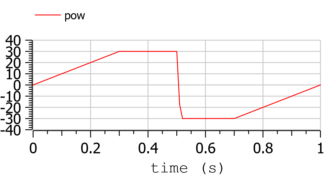
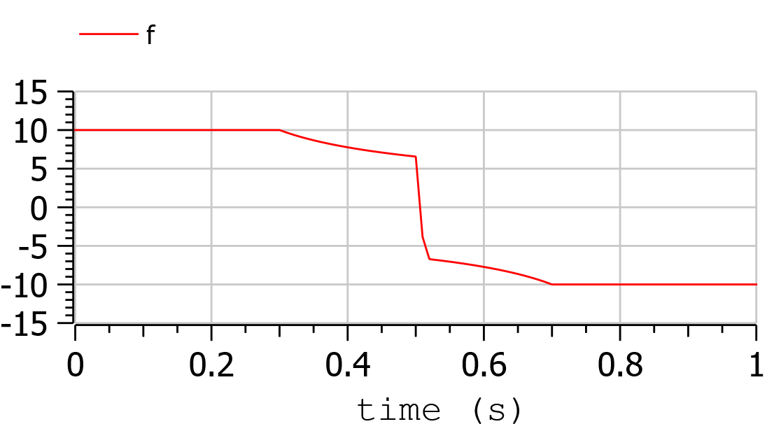
The results can be expressed in terms of force and power applied to the vehicle. They are as follows:

and they are as expected.

In this model we don't use the Modelica capability to automatically determine the system equations from the graphical description of a system. In other words, the above general formulation $0 = f\left( \mathbf{x}(t),\dot{\mathbf{x}}(t),\mathbf{u}(t),t \right)$ is explicitly written as follows:

der(pos) = v;
der(v) = a;

In the following example, we will use this capability extensively.

Example 2: hybrid vehicle minimum consumption¶

This example refers to the electricity generation of a hybrid vehicle. These vehicles can choose at any time which amount of the propulsion power must be taken from a battery and which from the Internal combustion engine.

In this example the engine can be switched ON and off without penalty, so the DO can choose both when the ICE must be ON /OFF; and the power it must deliver when it is ON.

Objective of the control is to minimise the fuel consumption. This must be done keeping the energy inside the storage at the final time, equal to the one at t=0 (otherwise it is easy to have zero consumption: just keep the Internal Combustion Engine OFF all the time!)

For simplicity's sake, the propulsion power, in this simple example is taken as being a sine wave plus an offset (needed to make the average positive). When the power is positive the wheels transfer power to the road, when negative they recover it (storing it into the battery).

To find the optimum, a fuel consumption curve is added, as follows:

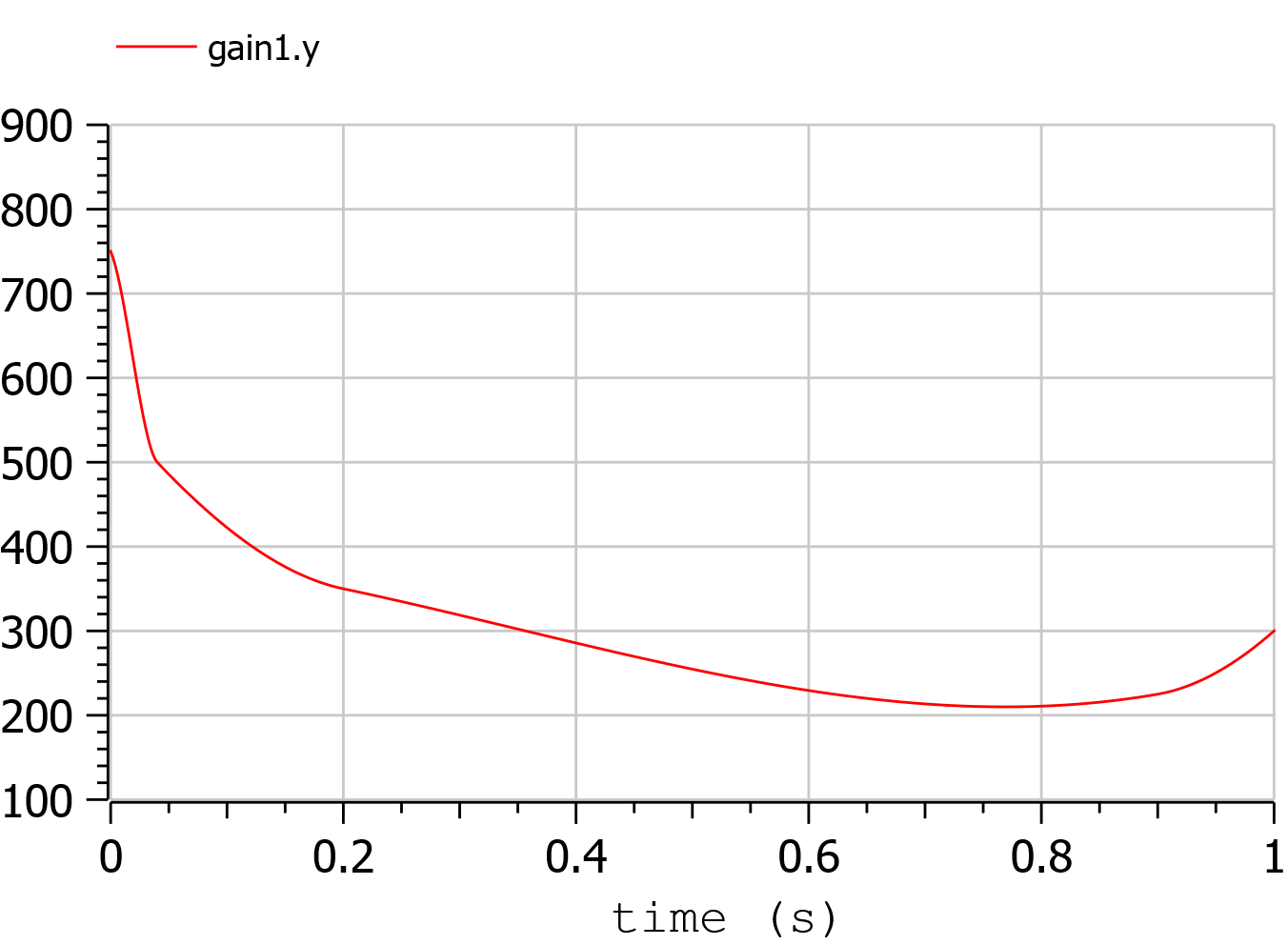
The minimum is 210 g/kWh, and occurs when the ICE power is at the 76.8 % of the nominal power

The system diagram is as follows

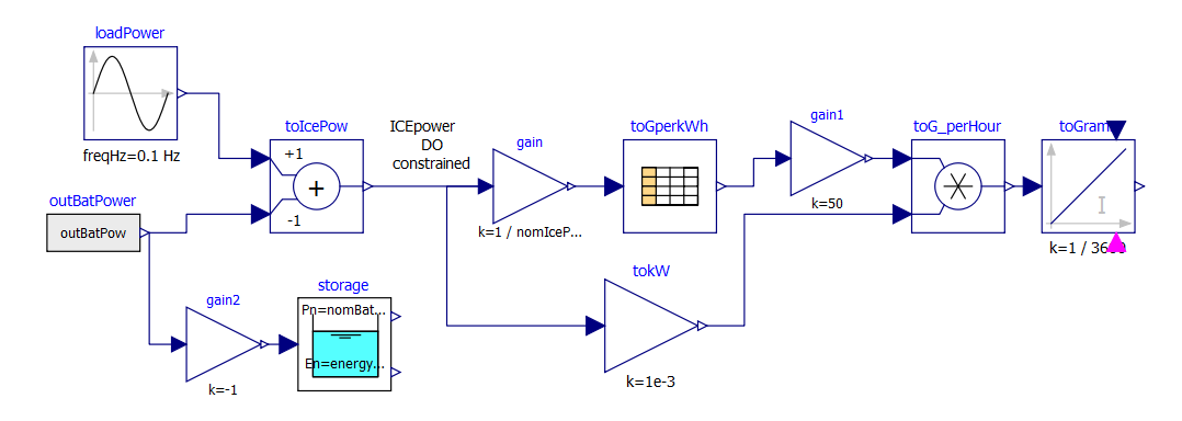
The DO algorithm is required to determine the battery power outBatPower (positive when the battery delivers power) so that to minimise the fuel consumption toGrams. Block toGperkWh is normalised, so that it can be used for different engines, adapting the horizontal scale through gain, and the vertical's through gain1.

This diagram defines the system, whose equations will be automatically determined by OpenModelica, through model flattening. However, some code must be manually written to perform DO.

Here the code is as follows:

//*** DO-related rows

input Real outBatPow;

//
Real totalCost = toGrams.y "minimize totalCost(tf)" annotation( isMayer=true);
//

Real energyConstr(min = 0, max = energyMax) = storage.energy annotation(isConstraint = true); //timespan constraint on storage energy

parameter Real fecp = 1 "final energy constraint parameter";

Real energyFinConstr(min = energyIni, max = energyIni) = fecp * storage.energy annotation(isFinalConstraint = true);//final time constraint on storage energy

Real icePowerConstr(min = 0) = itoIcePow.y annotation(isConstraint=true); //timespan constraint on Ice power

//*** End of DO-related rows

A few comments:

The choice isMayer=true on the objective function totalCost requires its final value to be actually minimised, not its integral (as would have been in case of the keyword isLaplace=true)
We have two different constraints on the storage energy: the storage energy must all the time be between 0 and the maximum allowed, and at the end of the simulation must be brought back to its initial value.
ICE can only deliver power, not absorb; so, we expect all the (regenerative) braking power and energy to be sent into the storage

Ideal storage¶

Here we consider the storage to be ideal: the flow of power in and out causes no losses to occur

In this case the solution of our optimization problem is trivial:

The Ice must supply the average power requested by the load, and when it does this it must do it at the optimal point which, as seen above is when its power is at the 76.8% of its nominal value
The battery supplies the load power minus ICE power.

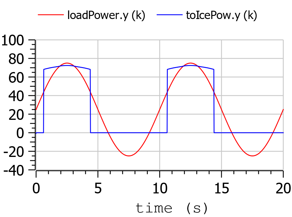
Using iceNominalPower=60 kW we get the following output:

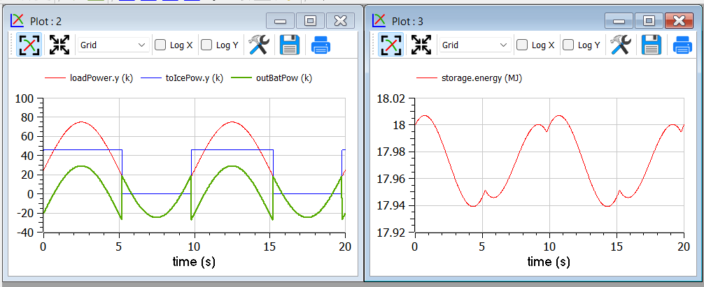
We see, as expected that the ICE is switched ON and OFF; and when it is ON it delivers at its 76.8 % of nominal power, i.e. at 46.1 kW. The battery delivers the difference, and when the load is negative absorbs all the power from it. The control is such that the energy at the end of the transient is the same as the one at t=0.

This result is good and confirms what we expected.

Effects of tolerance¶

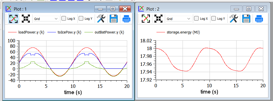
We mentioned that reduction of tolerance may affect the result adversely by large, especially when the minimum, as in this case is very flat (since the specific fuel consumption curve used for our example is very flat).

In the following picture we see the result of the previous section as it appears when we release tolerance by changing it from 1e-7 to and 1e-6. Now the result is badly wrong (and the total cost has changed from to 25.6g 29.9g).

More realistic storage¶

To the DO to be useful, it must obviously go beyond what is exactly expected. Therefore, we repeat the simulation adding the simulation of some losses inside the battery. According to scientific literature, losses here are modelled through the following formula:

$L(t) = 0.03{|P}_{\text{batt}}(t)| + 0.04\frac{P_{\text{batt}}^{2}(t)}{P_{batt,nom}}$

Which reflects that they in part are proportional to the absolute value of battery current, partly to its square. The coefficients are typical for power electronic converters interfacing a battery.

Inside the code, however, the formula introduced is structurally different, since it has been transformed to avoid the derivative discontinuity of the absolute value of a quantity around zero, using a trick like the one reported in sect. 1.4.

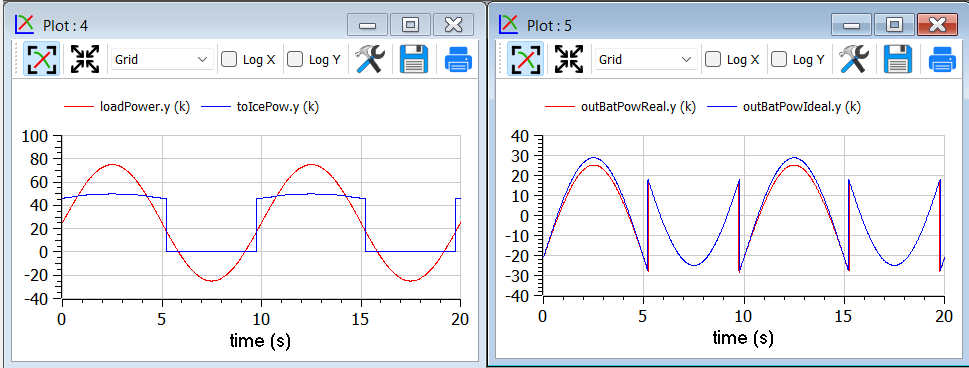
We see that now the optimiser changes the Ice power when in ON state, to reduce the battery power at its peak, since the losses formula pushes towards lower powers.

Adding storage power limitation¶

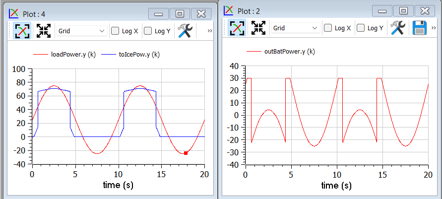
As a last case for example 2, we ass tome limitation on the power that can be exchanged by the battery. This can be physically due to limitations of either the battery or the inverter connected to it.

To show better the effect, we first rise the ICE power to 100 kW, so that the interval of ICE operation is smaller:

Then we change the following row of code:

input Real outBatPow;

into:

input Real outBatPow(min = -maxBatPower, max = maxBatPower);

where

parameter Modelica.SIunits.Power maxBatPower = 30e3;

giving rise to the following results (with a much longer computation time than in the previous cases):

Example 3: Acausal vehicle¶

As a last example, we replicate the optimization of Example 2, but the power to be delivered directly deriving from simulation of a vehicle, modelled through its physical elements.

The considered diagram is as follows:

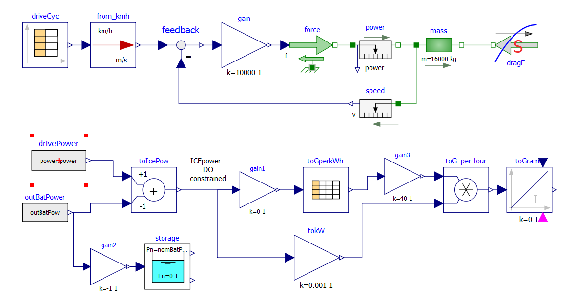
The upper part contains a vehicle model. The model follows a speed profile defined by the drive cycle driveCyc, through a simple proportional controller (simulating the driver). The power is applied to a mass; the drag force dragF sis the force against the movement due to friction (independent on speed) and air resistance (proportional to the square of vehicle speed).

The lower part contains the management of the storage, and the optimization algorithm, already discussed in example 2.

The results are shown in the following picture, where the obtained cost (red curve) is compared to what obtainable in case the ICE is continuously kept ON (blue curve), at a power (blue curve) that allows the battery energy at the end of the simulation to be equal to the one as t=0, as in the case of the optimised solution.

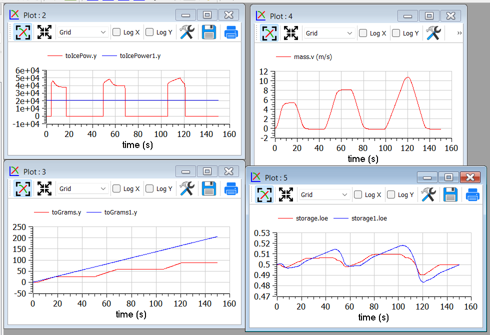
This example shows that the optimizer can find an ON/OFF strategy that more than halves the hybrid vehicle fuel consumption.

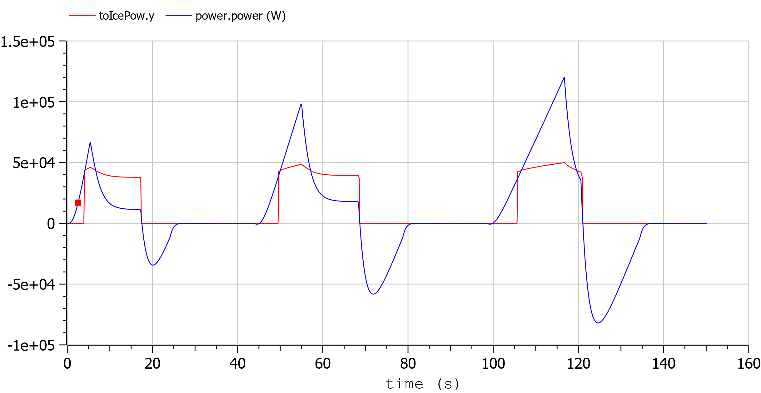
The following plot shows the ICE power in comparison with total power needed to cover the given trip profile mass.v. The rest is supplied by the battery.

Built-in Dynamic Optimization using Optimica language extensions¶

Note: this is a very short preliminary description which soon will be considerably improved.

OpenModelica provides builtin dynamic optimization of models by using the powerful symbolic machinery of the OpenModelica compiler for more efficient and automatic solution of dynamic optimization problems.

The builtin dynamic optimization allows users to define optimal control problems (OCP) using the Modelica language for the model and the optimization language extension called Optimica (currently partially supported) for the optimization part of the problem. This is used to solve the underlying dynamic optimization model formulation using collocation methods, using a single execution instead of multiple simulations as in the parameter-sweep optimization described in section Parameter Sweep Optimization using OMOptim.

For more detailed information regarding background and methods, see [BOR+12, RBB+14]

Before starting the optimization the model should be symbolically instantiated by the compiler in order to get a single flat system of equations. The model variables should also be scalarized. The compiler frontend performs this, including syntax checking, semantics and type checking, simplification and constant evaluation etc. are applied. Then the complete flattened model can be used for initialization, simulation and last but not least for model-based dynamic optimization.

The OpenModelica command optimize(ModelName) from OMShell, OMNotebook or MDT runs immediately the optimization. The generated result file can be read in and visualized with OMEdit or within OMNotebook.

An Example¶

In this section, a simple optimal control problem will be solved. When formulating the optimization problems, models are expressed in the Modelica language and optimization specifications. The optimization language specification allows users to formulate dynamic optimization problems to be solved by a numerical algorithm. It includes several constructs including a new specialized class optimization, a constraint section, startTime, finalTime etc. See the optimal control problem for batch reactor model below.

Create a new file named BatchReactor.mo and save it in you working directory. Notice that this model contains both the dynamic system to be optimized and the optimization specification.

Once we have formulated the undelying optimal control problems, we can run the optimization by using OMShell, OMNotebook, MDT, OMEdit using command line terminals similar to the options described below:

>>> setCommandLineOptions("-g=Optimica");

Listing 6 BatchReactor.mo¶

model BatchReactor
  Real x1(start =1, fixed=true, min=0, max=1);
  Real x2(start =0, fixed=true, min=0, max=1);
  input Real u(min=0, max=5);
equation
  der(x1) = -(u+u^2/2)*x1;
  der(x2) = u*x1;
end BatchReactor;

optimization nmpcBatchReactor(objective=-x2)
  extends BatchReactor;
end nmpcBatchReactor;

>>> optimize(nmpcBatchReactor, numberOfIntervals=16, stopTime=1, tolerance=1e-8)
record SimulationResult
    resultFile = "«DOCHOME»/nmpcBatchReactor_res.mat",
    simulationOptions = "startTime = 0.0, stopTime = 1.0, numberOfIntervals = 16, tolerance = 1e-8, method = 'optimization', fileNamePrefix = 'nmpcBatchReactor', options = '', outputFormat = 'mat', variableFilter = '.*', cflags = '', simflags = ''",
    messages = "LOG_SUCCESS       | info    | The initialization finished successfully without homotopy method.

Optimizer Variables
========================================================
State[0]:x1(start = 1, nominal = 1, min = 0, max = 1, init = 1)
State[1]:x2(start = 0, nominal = 1, min = 0, max = 1, init = 0)
Input[2]:u(start = 0, nominal = 5, min = 0, max = 5)
--------------------------------------------------------
number of nonlinear constraints: 0
========================================================

******************************************************************************
This program contains Ipopt, a library for large-scale nonlinear optimization.
 Ipopt is released as open source code under the Eclipse Public License (EPL).
         For more information visit https://github.com/coin-or/Ipopt
******************************************************************************

LOG_SUCCESS       | info    | The simulation finished successfully.
",
    timeFrontend = 0.065905133,
    timeBackend = 0.009299723000000001,
    timeSimCode = 0.0016700310000000002,
    timeTemplates = 0.0047043810000000005,
    timeCompile = 0.616270273,
    timeSimulation = 0.048362516,
    timeTotal = 0.746405598
end SimulationResult;

The control and state trajectories of the optimization results:

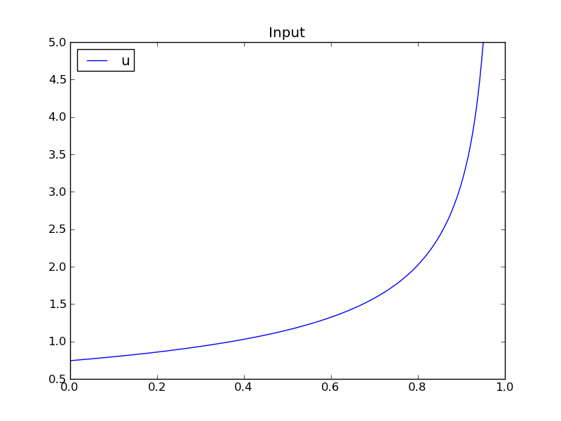
_images/nmpc-input.svg — Figure 86 Optimization results for Batch Reactor model - input variables.¶

_images/nmpc-states.svg — Figure 87 Optimization results for Batch Reactor model - state variables.¶

Table 1 New meanings of the usual simualtion options for Ipopt.¶
numberOfIntervals		collocation intervals
startTime, stopTime		time horizon
tolerance = 1e-8	e.g. 1e-8	solver tolerance
simflags	all run/debug options

Table 2 New simulation options for Ipopt.¶
-lv	LOG_IPOPT	console output
-ipopt_hesse	CONST,BFGS,NUM	hessian approximation
-ipopt_max_iter	number e.g. 10	maximal number of iteration for ipopt
externalInput.csv		input guess

Dynamic Optimization with OpenModelica and CasADi¶

OpenModelica coupling with CasADi supports dynamic optimization of models by OpenModelica exporting the optimization problem to CasADi which performs the optimization. In order to convey the dynamic system model information between Modelica and CasADi, we use an XML-based model exchange format for differential-algebraic equations (DAE). OpenModelica supports export of models written in Modelica and the Optimization language extension using this XML format, while CasADi supports import of models represented in this format. This allows users to define optimal control problems (OCP) using Modelica and Optimization language specifications, and solve the underlying model formulation using a range of optimization methods, including direct collocation and direct multiple shooting.

Before exporting a model to XML, the model should be symbolically instantiated by the compiler in order to get a single flat system of equations. The model variables should also be scalarized. The compiler frontend performs this, including syntax checking, semantics and type checking, simplification and constant evaluation etc. are applied. Then the complete flattened model is exported to XML code. The exported XML document can then be imported to CasADi for model-based dynamic optimization.

The OpenModelica command translateModelXML(ModelName) from OMShell, OMNotebook or MDT exports the XML. The export XML command is also integrated with OMEdit. Select XML > Export XML the XML document is generated in the current directory of omc. You can use the cd() command to see the current location. After the command execution is complete you will see that a file ModelName.xml has been exported.

Assuming that the model is defined in the modelName.mo, the model can also be exported to an XML code using the following steps from the terminal window:

Go to the path where your model file found
Run command omc -g=Optimica --simCodeTarget=XML Model.mo

In this section, a simple optimal control problem will be solved. When formulating the optimization problems, models are expressed in the Modelica language and optimization specifications. The optimization language specification allows users to formulate dynamic optimization problems to be solved by a numerical algorithm. It includes several constructs including a new specialized class optimization, a constraint section, startTime, finalTime etc. See the optimal control problem for batch reactor model below.

Create a new file named BatchReactor.mo and save it in you working directory. Notice that this model contains both the dynamic system to be optimized and the optimization specification.

>>> list(BatchReactor)
model BatchReactor
  Real x1(start = 1, fixed = true, min = 0, max = 1);
  Real x2(start = 0, fixed = true, min = 0, max = 1);
  input Real u(min = 0, max = 5);
equation
  der(x1) = -(u + u^2/2)*x1;
  der(x2) = u*x1;
end BatchReactor;

One we have formulated the underlying optimal control problems, we can export the XML by using OMShell, OMNotebook, MDT, OMEdit or command line terminals which are described in Section xml-import-to-casadi.

To export XML, we set the simulation target to XML:

>>> translateModelXML(BatchReactor)
"«DOCHOME»/BatchReactor.xml"

This will generate an XML file named BatchReactor.xml (Listing 7) that contains a symbolic representation of the optimal control problem and can be inspected in a standard XML editor.

Listing 7 BatchReactor.xml¶

<?xml version="1.0" encoding="UTF-8"?>
<OpenModelicaModelDescription
  xmlns:exp="https://github.com/JModelica/JModelica/tree/master/XML/daeExpressions.xsd"
  xmlns:equ="https://github.com/JModelica/JModelica/tree/master/XML/daeEquations.xsd"
  xmlns:fun="https://github.com/JModelica/JModelica/tree/master/XML/daeFunctions.xsd"
  xmlns:opt="https://github.com/JModelica/JModelica/tree/master/XML/daeOptimization.xsd"
  xmlns:xsi="http://www.w3.org/2001/XMLSchema-instance"
  fmiVersion="1.0"
  modelName="BatchReactor"
  modelIdentifier="BatchReactor"
  guid="{ff319e03-48a0-446f-918b-d4a514978011}"
  generationDateAndTime="2024-10-31T11:27:23"
  variableNamingConvention="structured"
  numberOfContinuousStates="2"
  numberOfEventIndicators="0"
  >
  
  <VendorAnnotations>
    <Tool name="OpenModelica Compiler OMCompiler v1.24.1-v1.24.1.2+ge6b7b28df0"> </Tool>
  </VendorAnnotations>


  <ModelVariables>
    <ScalarVariable name="x1"  valueReference="0" variability="continuous" causality="local" alias="noAlias">
      <Real start="1.0" fixed="true" min="0.0" max="1.0"  />
      <QualifiedName>
        <exp:QualifiedNamePart name="x1"/>
      </QualifiedName>
    <isLinearTimedVariables>
      <TimePoint index="0" isLinear="true"/>
    </isLinearTimedVariables>
      <VariableCategory>state</VariableCategory>
    </ScalarVariable>

    <ScalarVariable name="x2"  valueReference="1" variability="continuous" causality="local" alias="noAlias">
      <Real start="0.0" fixed="true" min="0.0" max="1.0"  />
      <QualifiedName>
        <exp:QualifiedNamePart name="x2"/>
      </QualifiedName>
    <isLinearTimedVariables>
      <TimePoint index="0" isLinear="true"/>
    </isLinearTimedVariables>
      <VariableCategory>state</VariableCategory>
    </ScalarVariable>
    <ScalarVariable name="der(x1)"  valueReference="2" variability="continuous" causality="local" alias="noAlias">
      <Real     />
      <QualifiedName>
        <exp:QualifiedNamePart name="x1"/>
      </QualifiedName>
    <isLinearTimedVariables>
      <TimePoint index="0" isLinear="true"/>
    </isLinearTimedVariables>
      <VariableCategory>derivative</VariableCategory>
    </ScalarVariable>

    <ScalarVariable name="der(x2)"  valueReference="3" variability="continuous" causality="local" alias="noAlias">
      <Real     />
      <QualifiedName>
        <exp:QualifiedNamePart name="x2"/>
      </QualifiedName>
    <isLinearTimedVariables>
      <TimePoint index="0" isLinear="true"/>
    </isLinearTimedVariables>
      <VariableCategory>derivative</VariableCategory>
    </ScalarVariable>
    <ScalarVariable name="u"  valueReference="4" variability="continuous" causality="input" alias="noAlias">
      <Real  min="0.0" max="5.0"  />
      <QualifiedName>
        <exp:QualifiedNamePart name="u"/>
      </QualifiedName>
    <isLinearTimedVariables>
      <TimePoint index="0" isLinear="true"/>
    </isLinearTimedVariables>
      <VariableCategory>algebraic</VariableCategory>
    </ScalarVariable>
  </ModelVariables>

  <equ:BindingEquations>
  </equ:BindingEquations>

  <equ:DynamicEquations>
    <equ:Equation>
      <exp:Sub>
        <exp:Der>
          <exp:Identifier>
            <exp:QualifiedNamePart name="x2"/>
          </exp:Identifier>
        </exp:Der>
        <exp:Mul>
          <exp:Identifier>
            <exp:QualifiedNamePart name="u"/>
          </exp:Identifier>
          <exp:Identifier>
            <exp:QualifiedNamePart name="x1"/>
          </exp:Identifier>
        </exp:Mul>
      </exp:Sub>
    </equ:Equation>
    <equ:Equation>
      <exp:Sub>
        <exp:Der>
          <exp:Identifier>
            <exp:QualifiedNamePart name="x1"/>
          </exp:Identifier>
        </exp:Der>
        <exp:Mul>
          <exp:Sub>
            <exp:Mul>
              <exp:RealLiteral>-0.5</exp:RealLiteral>
              <exp:Pow>
                <exp:Identifier>
                  <exp:QualifiedNamePart name="u"/>
                </exp:Identifier>
                <exp:RealLiteral>2.0</exp:RealLiteral>
              </exp:Pow>
            </exp:Mul>
            <exp:Identifier>
              <exp:QualifiedNamePart name="u"/>
            </exp:Identifier>
          </exp:Sub>
          <exp:Identifier>
            <exp:QualifiedNamePart name="x1"/>
          </exp:Identifier>
        </exp:Mul>
      </exp:Sub>
    </equ:Equation>
  </equ:DynamicEquations>

  <equ:InitialEquations>
    <equ:Equation>
      <exp:Sub>
        <exp:Identifier>
          <exp:QualifiedNamePart name="x1"/>
        </exp:Identifier>
        <exp:RealLiteral>1.0</exp:RealLiteral>
      </exp:Sub>
    </equ:Equation>

    <equ:Equation>
      <exp:Sub>
        <exp:Identifier>
          <exp:QualifiedNamePart name="x2"/>
        </exp:Identifier>
        <exp:RealLiteral>0.0</exp:RealLiteral>
      </exp:Sub>
    </equ:Equation>
    <equ:Equation>
      <exp:Sub>
        <exp:Identifier>
          <exp:QualifiedNamePart name="x1"/>
        </exp:Identifier>
        <exp:Identifier>
          <exp:QualifiedNamePart name="$START"/>
          <exp:QualifiedNamePart name="x1"/>
        </exp:Identifier>
      </exp:Sub>
    </equ:Equation>
    <equ:Equation>
      <exp:Sub>
         
      </exp:Sub>
    </equ:Equation>
    <equ:Equation>
      <exp:Sub>
         
      </exp:Sub>
    </equ:Equation>
    <equ:Equation>
      <exp:Sub>
        <exp:Identifier>
          <exp:QualifiedNamePart name="x2"/>
        </exp:Identifier>
        <exp:Identifier>
          <exp:QualifiedNamePart name="$START"/>
          <exp:QualifiedNamePart name="x2"/>
        </exp:Identifier>
      </exp:Sub>
    </equ:Equation>
  </equ:InitialEquations>

  <fun:Algorithm>
  </fun:Algorithm>

  <fun:RecordsList>
  </fun:RecordsList>

  <fun:FunctionsList>
  </fun:FunctionsList>

  <opt:Optimization>
    <opt:TimePoints>
      <opt:TimePoint  >
      </opt:TimePoint>
    </opt:TimePoints>
    <opt:PathConstraints>
    </opt:PathConstraints>
  </opt:Optimization>

</OpenModelicaModelDescription>

The symbolic optimal control problem representation (or just model description) contained in BatchReactor.xml can be imported into CasADi in the form of the SymbolicOCP class via OpenModelica python script.

The SymbolicOCP class contains symbolic representation of the optimal control problem designed to be general and allow manipulation. For a more detailed description of this class and its functionalities, we refer to the API documentation of CasADi.

The following step compiles the model to an XML format, imports to CasADi and solves an optimization problem in windows PowerShell:

Create a new file named BatchReactor.mo and save it in you working directory.

E.g. C:\OpenModelica1.9.2\share\casadi\testmodel
Perform compilation and generate the XML file
1. Go to your working directory
E.g. cd C:\OpenModelica1.9.2\share\casadi\testmodel

Go to omc path from working directory and run the following command

E.g. ..\..\..\bin\omc +s -g=Optimica --simCodeTarget=XML BatchReactor.mo

3. Run defaultStart.py python script from OpenModelica optimization directory

E.g. Python.exe ..\share\casadi\scripts defaultStart.py BatchReactor.xml

The control and state trajectories of the optimization results are shown below:

Parameter Sweep Optimization using OMOptim¶

OMOptim is a tool for parameter sweep design optimization of Modelica models. By optimization, one should understand a procedure which minimizes/maximizes one or more objective functions by adjusting one or more parameters. This is done by the optimization algorithm performing a parameter swep, i.e., systematically adjusting values of selected parameters and running a number of simulations for different parameter combinations to find a parameter setting that gives an optimal value of the goal function.

OMOptim 0.9 contains meta-heuristic optimization algorithms which allow optimizing all sorts of models with following functionalities:

One or several objectives optimized simultaneously
One or several parameters (integer or real variables)

However, the user must be aware of the large number of simulations an optimization might require.

Before launching OMOptim, one must prepare the model in order to optimize it.

An optimization parameter is picked up from all model variables. The choice of parameters can be done using the OMOptim interface.

For all intended parameters, please note that:

The corresponding variable is constant during all simulations.
The OMOptim optimization in version 0.9 only concerns static parameters' optimization i.e. values found for these parameters will be constant during all simulation time.
The corresponding variable should play an input role in the model
i.e. its modification influences model simulation results.

Constraints¶

If some constraints should be respected during optimization, they must be defined in the Modelica model itself.

For instance, if mechanical stress must be less than 5 N.m^-2, one should write in the model:

assert(mechanicalStress < 5, "Mechanical stress too high");

If during simulation, the variable mechanicalStress exceeds 5 N.m^-2, the simulation will stop and be considered as a failure.

Objectives¶

As parameters, objectives are picked up from model variables. Objectives' values are considered by the optimizer at the final time.

Set problem in OMOptim¶

Launch OMOptim¶

OMOptim can be launched using the executable placed in OpenModelicaInstallationDirectory/bin/ OMOptim/OMOptim.exe. Alternately, choose OpenModelica > OMOptim from the start menu.

Create a new project¶

To create a new project, click on menu File -> New project

Then set a name to the project and save it in a dedicated folder. The created file created has a .min extension. It will contain information regarding model, problems, and results loaded.

Load models¶

First, you need to load the model(s) you want to optimize. To do so, click on Add .mo button on main window or select menu Model -> Load Mo file…

When selecting a model, the file will be loaded in OpenModelica which runs in the background.

While OpenModelica is loading the model, you could have a frozen interface. This is due to multi-threading limitation but the delay should be short (few seconds).

You can load as many models as you want.

If an error occurs (indicated in log window), this might be because:

Dependencies have not been loaded before (e.g. modelica library)
Model use syntax incompatible with OpenModelica.

OMOptim should detect dependencies and load corresponding files. However, it some errors occur, please load by yourself dependencies. You can also load Modelica library using Model->Load Modelica library.

When the model correctly loaded, you should see a window similar to Figure 88.

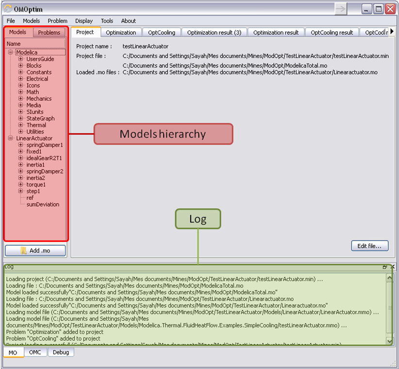
_images/omoptim-loaded.png — Figure 88 OMOptim window after having loaded model.¶

Create a new optimization problem¶

Problem->Add Problem->Optimization

A dialog should appear. Select the model you want to optimize. Only Model can be selected (no Package, Component, Block…).

A new form will be displayed. This form has two tabs. One is called Variables, the other is called Optimization.

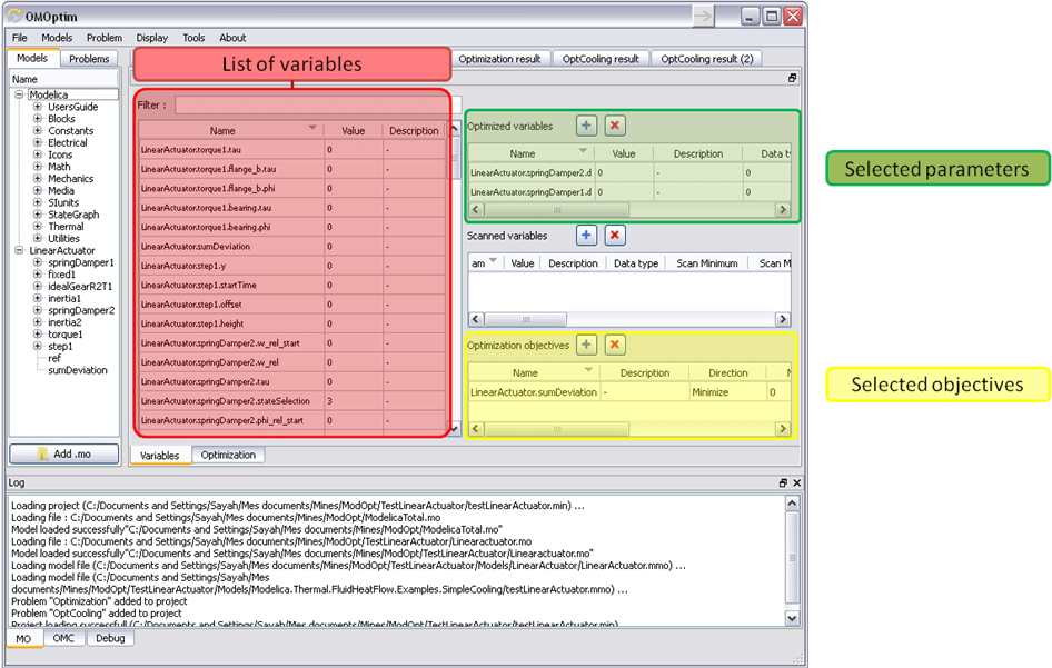
_images/omoptim-define-new-problem.png — Figure 89 Forms for defining a new optimization problem.¶

If variables are not displayed, right click on model name in model hierarchy, and select Read variables.

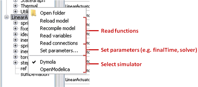
_images/omoptim-setup-model.png — Figure 90 Selecting read variables, set parameters, and selecting simulator.¶

Select Optimized Variables¶

To set optimization, we first have to define the variables the optimizer will consider as free i.e. those that it should find best values of. To do this, select in the left list, the variables concerned. Then, add them to Optimized variables by clicking on corresponding button ().

For each variable, you must set minimum and maximum values it can take. This can be done in the Optimized variables table.

Select objectives¶

Objectives correspond to the final values of chosen variables. To select these last, select in left list variables concerned and click button of Optimization objectives table.

For each objective, you must:

Set minimum and maximum values it can take. If a configuration does
not respect these values, this configuration won't be considered. You also can set minimum and maximum equals to “-“ : it will then
Define whether objective should be minimized or maximized.

This can be done in the Optimized variables table.

Select and configure algorithm¶

After having selected variables and objectives, you should now select and configure optimization algorithm. To do this, click on Optimization tab.

Here, you can select optimization algorithm you want to use. In version 0.9, OMOptim offers three different genetic algorithms. Let's for example choose SPEA2Adapt which is an auto-adaptative genetic algorithm.

By clicking on parameters… button, a dialog is opened allowing defining parameters. These are:

Population size: this is the number of configurations kept after a
generation. If it is set to 50, your final result can't contain more than 50 different points.
Off spring rate: this is the number of children per adult obtained
after combination process. If it is set to 3, each generation will contain 150 individual (considering population size is 50).
Max generations: this number defines the number of generations
after which optimization should stop. In our case, each generation corresponds to 150 simulations. Note that you can still stop optimization while it is running by clicking on stop button (which will appear once optimization is launched). Therefore, you can set a really high number and still stop optimization when you want without losing results obtained until there.
Save frequency: during optimization, best configurations can be
regularly saved. It allows to analyze evolution of best configurations but also to restart an optimization from previously obtained results. A Save Frequency parameter set to 3 means that after three generations, a file is automatically created containing best configurations. These files are named iteraion1.sav, iteration2.sav and are store in Temp directory, and moved to SolvedProblems directory when optimization is finished.
ReinitStdDev: this is a specific parameter of EAAdapt1. It defines
whether standard deviation of variables should be reinitialized. It is used only if you start optimization from previously obtained configurations (using Use start file option). Setting it to yes (1) will, in most of cases, lead to a spread research of optimized configurations, forgetting parameters' variations' reduction obtained in previous optimization.

As indicated before, it is possible to pursue an optimization finished or stopped. To do this, you must enable Use start file option and select file from which optimization should be started. This file is an iteration_.sav file created in previous optimization. It is stored in corresponding SolvedProblems folder (iteration10.sav corresponds to the tenth generation of previous optimization).

*Note that this functionality can only work with same variables and objectives*. However, minimum, maximum of variables and objectives can be changed before pursuing an optimization.

Launch¶

You can now launch Optimization by clicking Launch button.

Stopping Optimization¶

Optimization will be stopped when the generation counter will reach the generation number defined in parameters. However, you can still stop the optimization while it is running without loosing obtained results. To do this, click on Stop button. Note that this will not immediately stop optimization: it will first finish the current generation.

This stop function is especially useful when optimum points do not vary any more between generations. This can be easily observed since at each generation, the optimum objectives values and corresponding parameters are displayed in log window.

Results¶

The result tab appear when the optimization is finished. It consists of two parts: a table where variables are displayed and a plot region.

Obtaining all Variable Values¶

During optimization, the values of optimized variables and objectives are memorized. The others are not. To get these last, you must recomputed corresponding points. To achieve this, select one or several points in point's list region and click on recompute.

For each point, it will simulate model setting input parameters to point corresponding values. All values of this point (including those which are not optimization parameters neither objectives).

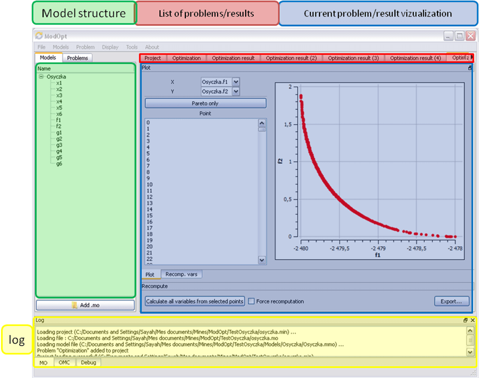
_images/omoptim-window-regions.png — Figure 91 Window regions in OMOptim GUI.¶

[BOR+12]

Bernhard Bachmann, Lennart Ochel, Vitalij Ruge, Mahder Gebremedhin, Peter Fritzson, Vaheed Nezhadali, Lars Eriksson, and Martin Sivertsson. Parallel multiple-shooting and collocation Optimization with OpenModelica. In Martin Otter and Dirk Zimmer, editors, Proceedings of the 9th International Modelica Conference. Linköping University Electronic Press, September 2012. doi:10.3384/ecp12076659.

[RBB+14]

Vitalij Ruge, Willi Braun, Bernhard Bachmann, Andrea Walther, and Kshitij Kulshreshtha. Efficient implementation of collocation methods for optimization using openmodelica and adol-c. In Hubertus Tummescheit and Karl-Erik Årzén, editors, Proceedings of the 10th International Modelica Conference. Modelica Association and Linköping University Electronic Press, March 2014. doi:10.3384/ecp140961017.